VPN-based security solutions
VPN-based security solutions are increasingly popular and have proven effective and secure technology for protecting sensitive data traversing insecure channel mediums, such as the Internet.
Traditional IPsec-based site-to-site, hub-to-spoke VPN deployment models must scale better and be adequate only for small- and medium-sized networks. However, as demand for IPsec-based VPN implementation grows, organizations with large-scale enterprise networks require scalable and dynamic IPsec solutions that interconnect sites across the Internet with reduced latency while optimizing network performance and bandwidth utilization.
Scaling traditional IPsec VPN
Dynamic Multipoint VPN (DMVPN) technology scales IPsec VPN networks by offering a large-scale deployment model that allows the network to expand and realize its full potential. In addition, DMVPN offers scalability that enables zero-touch deployment models.
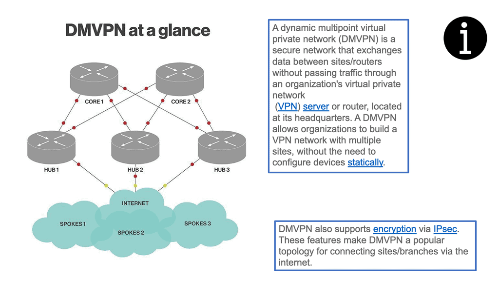
Encryption is supported through IPsec, making DMVPN a popular choice for connecting different sites using regular Internet connections. It’s a great backup or alternative to private networks like MPLS VPN. A popular option for DMVPN is FlexVPN.
Routing Technique
DMVPN (Dynamic Multipoint VPN) is a routing technique for building a VPN network with multiple sites without configuring all devices statically. It’s a “hub and spoke” network in which the spokes can communicate directly without going through the hub.
Advanced:
DMVPN Phase 2
DMVPN Phase 2 is an enhanced version of the initial DMVPN implementation. It introduces the concept of Next Hop Resolution Protocol (NHRP), which provides dynamic mapping between the participating devices’ physical and virtual IP addresses. This dynamic mapping allows for efficient and scalable communication within the DMVPN network.
Resolutions triggered by the NHRP
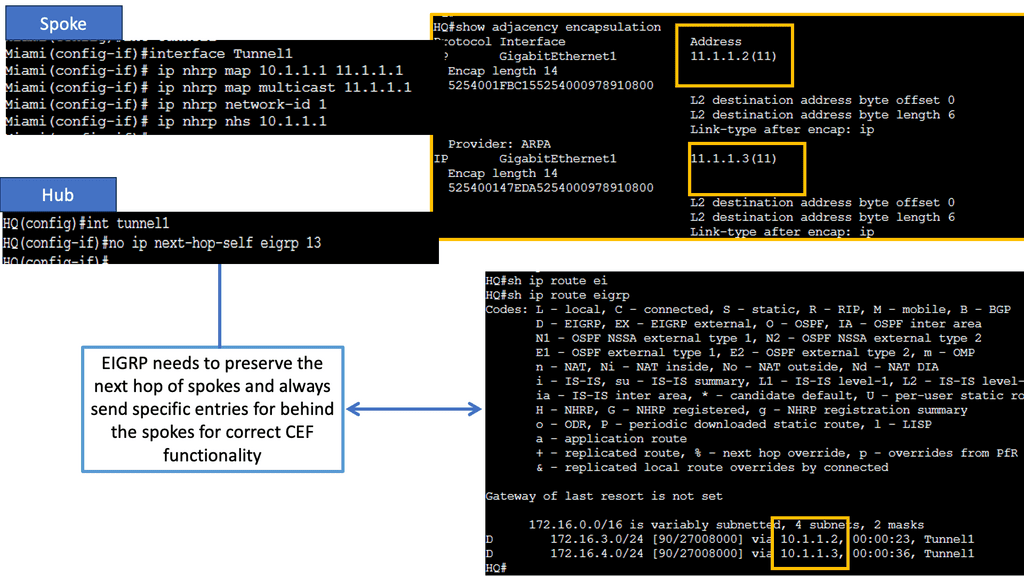
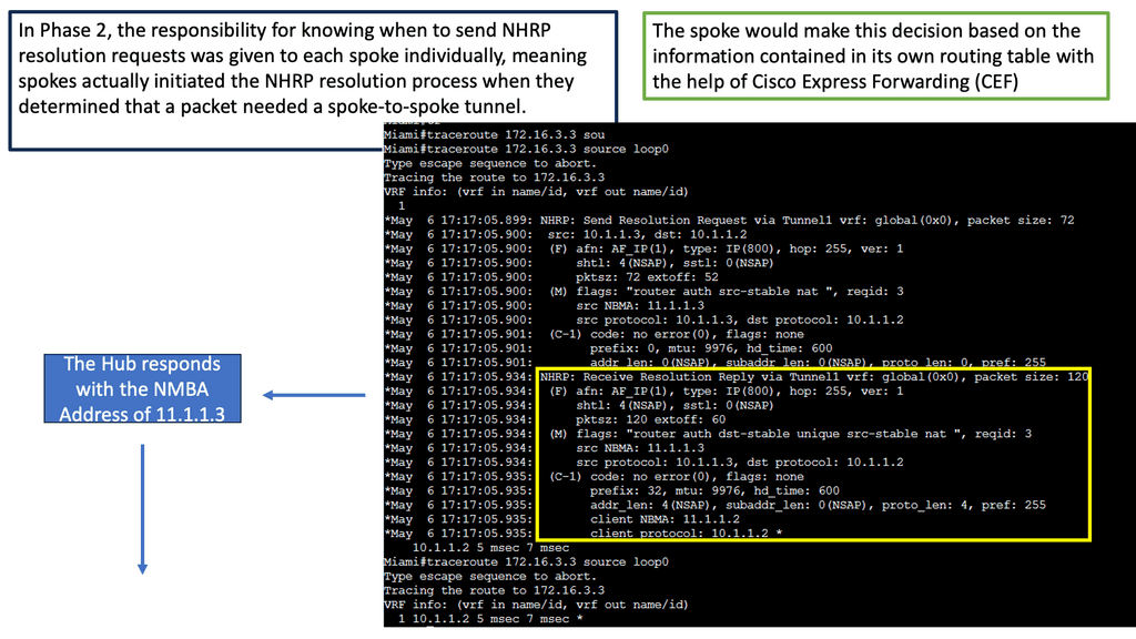
Learning the mapping information required through NHRP resolution creates a dynamic spoke-to-spoke tunnel. How does a spoke know how to perform such a task? As an enhancement to DMVPN Phase 1, spoke-to-spoke tunnels were first introduced in Phase 2 of the network. Phase 2 handed responsibility for NHRP resolution requests to each spoke individually, which means that spokes initiated NHRP resolution requests when they determined a packet needed a spoke-to-spoke tunnel.
Cisco Express Forwarding (CEF) would assist the spoke in making this decision based on information contained in its routing table.
Related: For pre-information, you may find the following posts helpful.
Cisco DMVPN
♦DMVPN Components Involved
The DMVPN solution consists of a combination of existing technologies so that sites can learn about each other and create dynamic VPNs. Therefore, efficiently designing and implementing a Cisco DMVPN network requires thoroughly understanding these components, their interactions, and how they all come together to create a DMVPN network.
These technologies may seem complex, and this post aims to simplify them. First, we mentioned that DMVPN has different components, which are the building blocks of a DMVPN network. These include Generic Routing Encapsulation (GRE), Next Hop Redundancy Protocol (NHRP), and IPsec.
The Dynamic Multipoint VPN (DMVPN) feature allows users to better scale large and small IP Security (IPsec) Virtual Private Networks (VPNs) by combining generic routing encapsulation (GRE) tunnels, IPsec encryption, and Next Hop Resolution Protocol (NHRP).
Each of these components needs a base configuration for DMVPN to work. Once the base configuration is in place, we have a variety of show and debug commands to troubleshoot a DMVPN network to ensure smooth operations.
There are four pieces to DMVPN:
- Multipoint GRE (mGRE)
- NHRP (Next Hop Resolution Protocol)
- Routing (RIP, EIGRP, OSPF, BGP, etc.)
- IPsec (not required but recommended)
Cisco DMVPN Components | Main DMVPN Components Dynamic VPN
|
1st Lab Guide: Displaying the DMVPN configuration
DMVPN Network
The following screenshot is from a DMVPN network using Cisco modeling labs. We have R1 as the hub, R2 and R3 as the spokes. The command: show DMVPN displays that we have two spokes routers. Notice the “D” attribute. This means the spokes have been learned dynamically, which is the essence of DMVPN.
The spokes are learned with a process called the Next Hop Resolution Protocol. As this is a nonbroadcast multiaccess network, we must use a protocol other than the Address Resolution Protocol (ARP).
Note:
- As you can see, with tunnel configuration for one of the spokes, we have a static mapping for the hub with the command IP nhrp NHS 192.168.100.1. We also have point-to-point GRE tunnels in the spokes with the command: tunnel destination 172.17.11.2.
- Therefore, we are running DMVPN Phase 1. DMVPN phase 3 will have mGRE. More on this later.
Key DMVPN components include:
● Multipoint GRE (mGRE) tunnel interface: Allows a single GRE interface to support multiple IPsec tunnels, simplifying the size and complexity of the configuration. Standard point-to-point GRE tunnels are used in the earlier versions or phases of DMVPN.
● Dynamic discovery of IPsec tunnel endpoints and crypto profiles: Eliminates the need to configure static crypto maps defining every pair of IPsec peers, further simplifying the configuration.
● NHRP: Allows spokes to be deployed with dynamically assigned public IP addresses (i.e., behind an ISP’s router). The hub maintains an NHRP database of the public interface addresses of each spoke. Each spoke registers its actual address when it boots; when it needs to build direct tunnels with other spokes, it queries the NHRP database for real addresses of the destination spokes
DMVPN Explained
Overlay Networking
A Cisco DMVPN network consists of many overlay virtual networks. Such a virtual network is called an overlay network because it depends on an underlying transport called the underlay network. The underlay network forwards traffic flowing through the overlay network. With the use of protocol analyzers, the underlay network is aware of the existence of the overlay. However, left to its defaults, the underlay network does not fully see the overlay network.
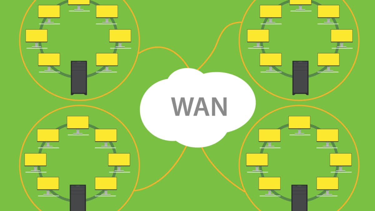
We will have routers at the company’s sites that are considered the endpoints of the tunnel that forms the overlay network. So, we could have a WAN edge router or Cisco ASA configured for DMVPN. Then, for the underlay that is likely out of your control, have an array of service provider equipment such as routers, switches, firewalls, and load balancers that make up the underlay.
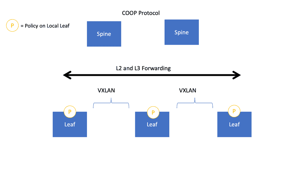
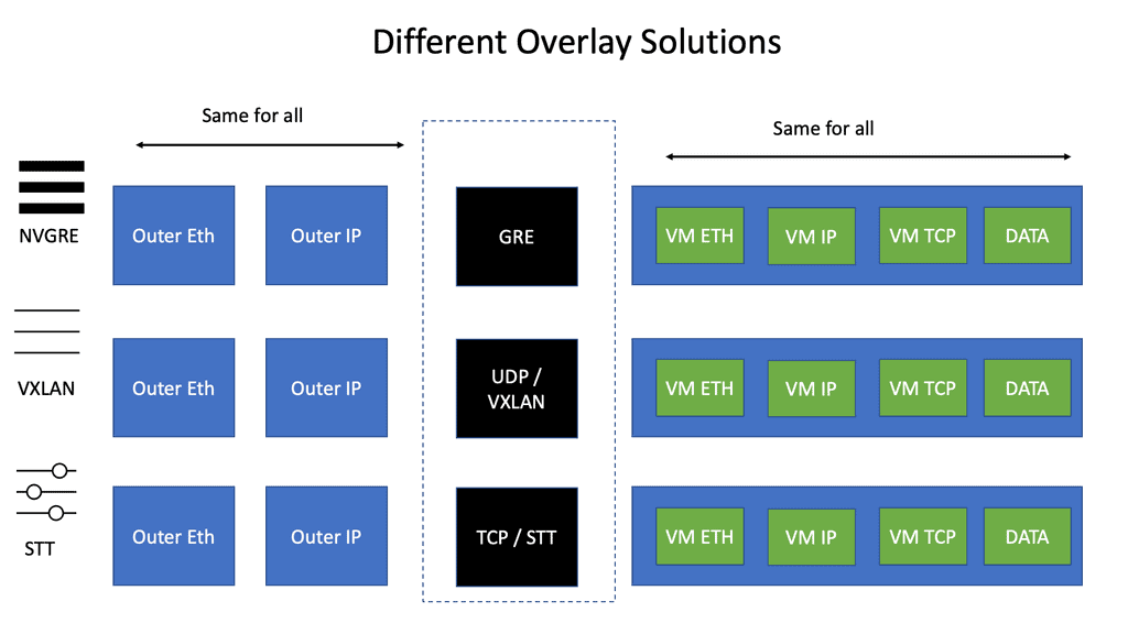
The following diagram displays the different overlay solutions. VXLAN is expected in the data center, while GRE is used across the WAN. DMVPN uses GRE.
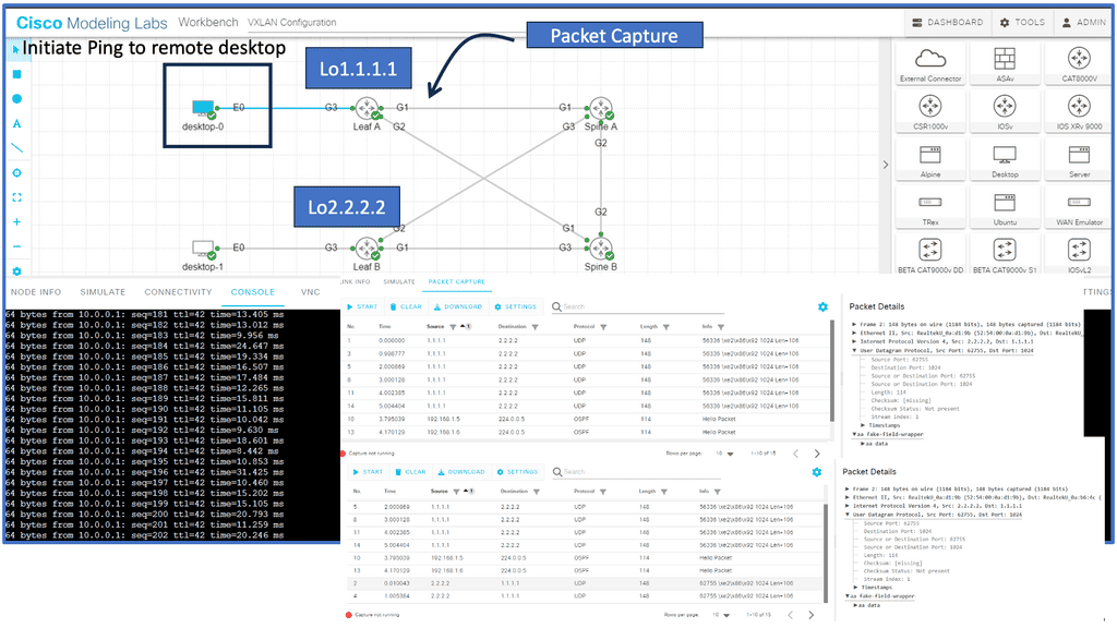
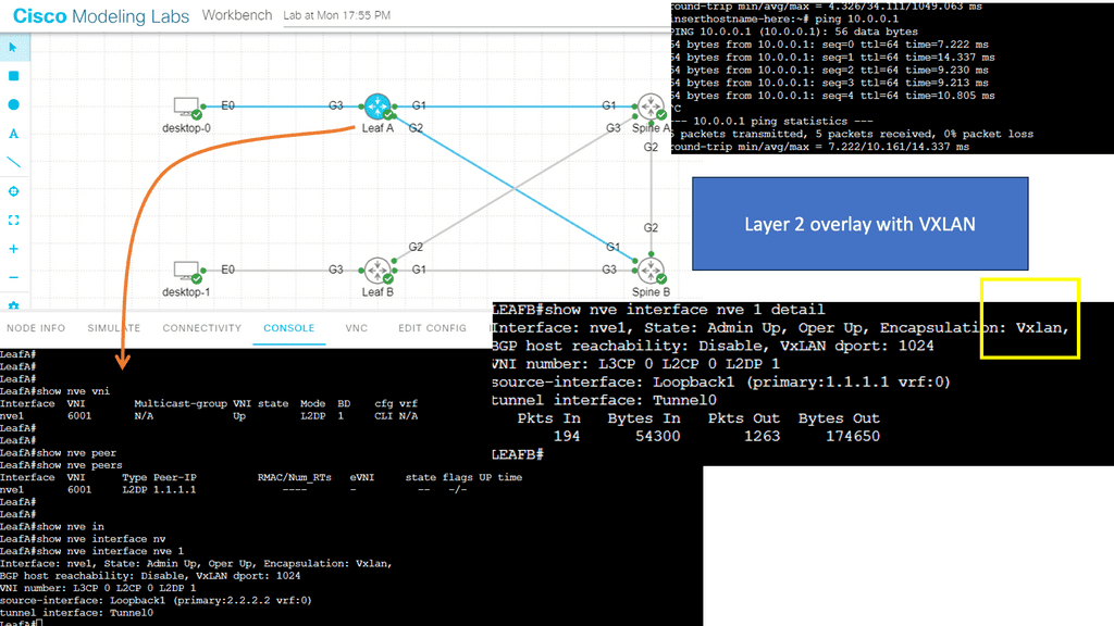
2nd Lab Guide: VXLAN overlay
Overlay Networking
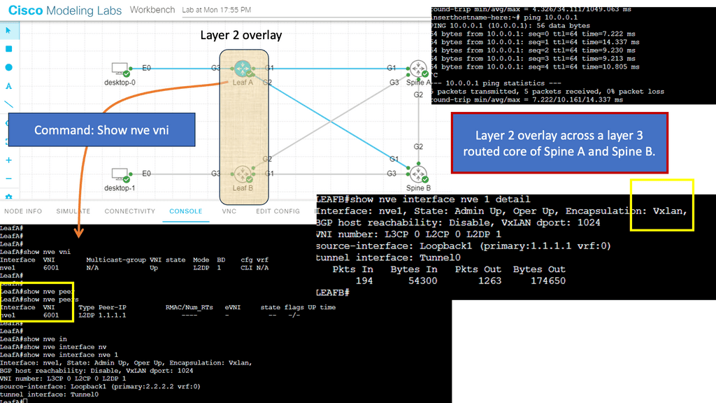
While DMVPN does not run VXLAN as the overlay protocol, viewing for background information and reference is helpful. VXLAN is a network overlay technology that provides a scalable and flexible solution for creating virtualized networks.
It enables the creation of logical Layer 2 networks over an existing Layer 3 infrastructure, allowing organizations to extend their networks across data centers and virtualized environments. In the following example, we create a Layer 2 overlay over a Layer 3 core. A significant difference between DMVPN’s use of GRE as the overlay and the use of VXLAN is the VNI.
Note:
- One critical component of VXLAN is the Virtual Network Identifier (VNI). In this blog post, we will explore the details of VXLAN VNI and its significance in modern network architectures.
- VNI is a 24-bit identifier that uniquely identifies a VXLAN network. It allows multiple VXLAN networks to coexist over the same physical network infrastructure. Each VNI represents a separate Layer 2 network, enabling the isolation and segmentation of traffic between different virtual networks.
Below, you can see the VNI used and the peers that have been created. VXLAN also works in multicast mode.
DMVPN Overlay Networking Creating an overlay network |
|
DMVPN: Creating an overlay network
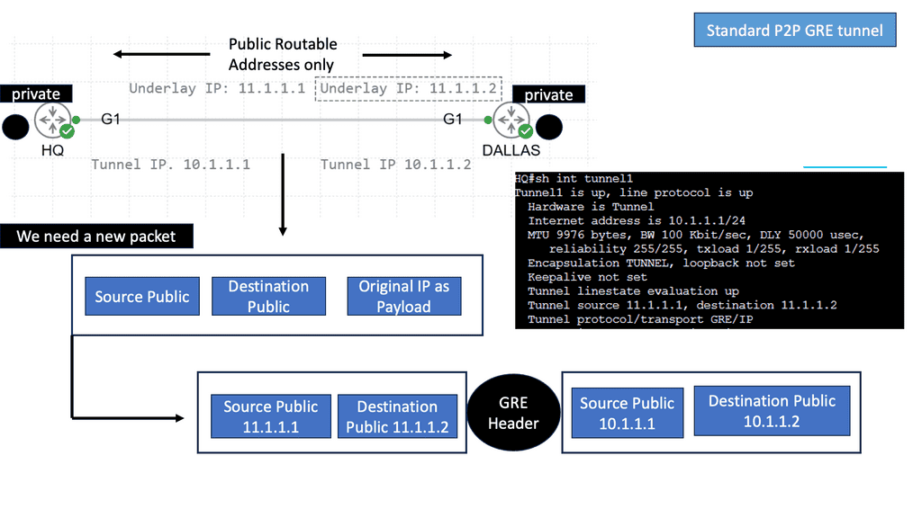
The overlay network does not magically appear. To create one, we need a tunneling technique. Many tunneling technologies can be used to form the overlay network. The Generic Routing Encapsulation (GRE) tunnel is the most widely used external connectivity, while VXLAN is used for internal connectivity to the data center.
And the one that DMVPN adopts. A GRE tunnel can support tunneling for various protocols over an IP-based network. It works by inserting an IP and GRE header on top of the original protocol packet, creating a new GRE/IP packet.
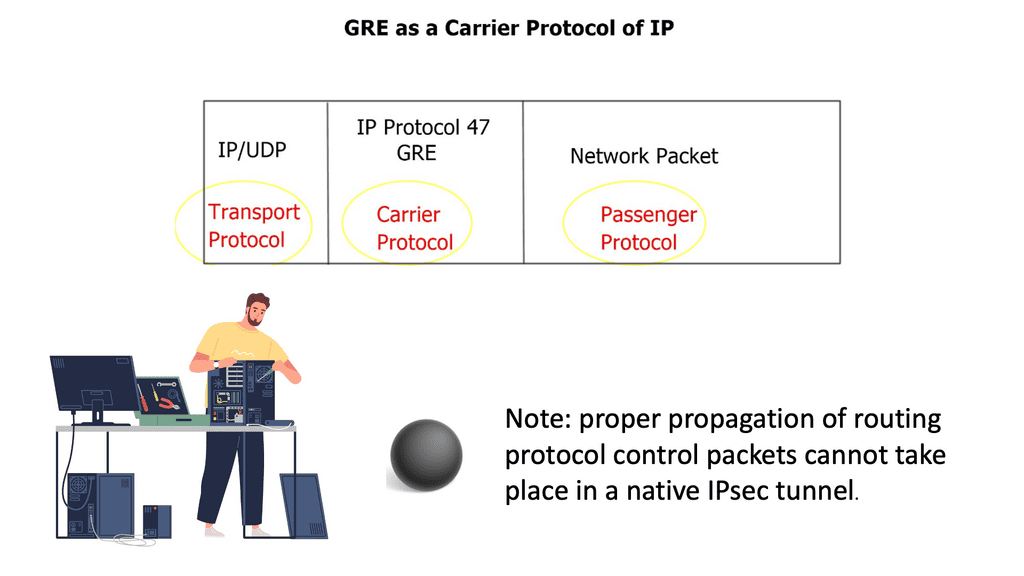
The resulting GRE/IP packet uses a source/destination pair routable over the underlying infrastructure. The GRE/IP header is the outer header, and the original protocol header is the inner header.
♦ Is GRE over IPsec a tunneling protocol?
GRE is a tunneling protocol that transports multicast, broadcast, and non-IP packets like IPX. IPSec is an encryption protocol. IPSec can only transport unicast packets, not multicast & broadcast. Hence, we wrap it GRE first and then into IPSec, which is called GRE over IPSec.
3rd Lab Guide: Displaying the DMVPN configuration
DMVPN Configuration
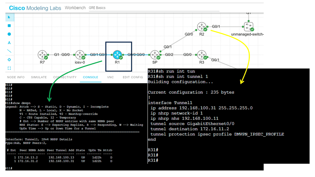
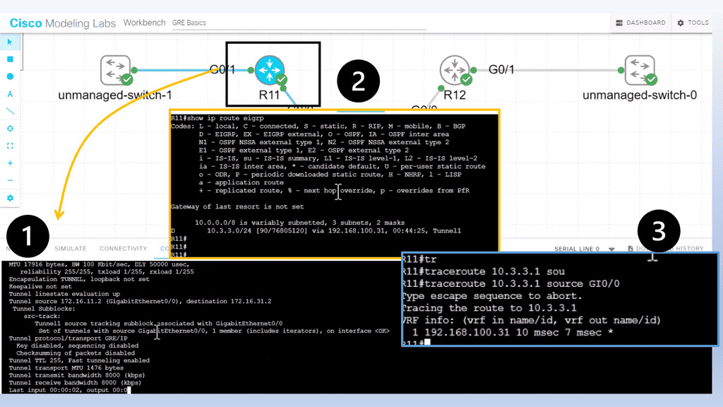
We are using a different DMVPN lab setup than before. R11 is the hub of the DMVPN network, and we only have one spoke of R12. In the DMVPN configuration, the tunnel interface has an “encapsulation tunnel.” This is the overlay network, and we are using GRE.
We are currently using the standard point-to-point GRE and not multipoint GRE. We know this as we have explicitly set the tunnel destination with the command tunnel destination 172.16.31.2. This is fine for a small network of a few spokes. However, for the more extensive network, we need to use mGRE. And take full advantage of the dynamic nature of DMVPN.
Note:
- As for the routing protocols, we run EIGRP over the tunnel ( GRE ) interface. So, we only have one EIGRP neighbor, so we don’t need to worry about the split horizon. Before we move on, one key point is that running a traceroute from R11 to R12 only shows one hop.
- This is because the TTL is also carried in the GRE. So, no matter how many devices are in the path ( underlay network ) between R11 and R12, either physical or virtual, it will always show as one hop due to the overlay network, i.e., GRE.
Multipoint GRE. What is mGRE?
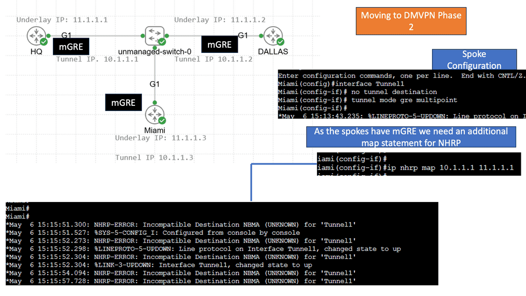
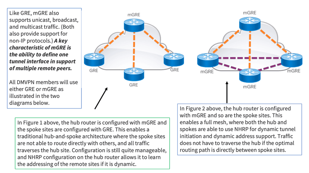
An alternative to configuring multiple point-to-point GRE tunnels is to use multipoint GRE tunnels to provide the connectivity desired. Multipoint GRE (mGRE) tunnels are similar in construction to point-to-point GRE tunnels except for the tunnel destination command. However, instead of declaring a static destination, no destination is declared, and instead, the tunnel mode gre multipoint command is issued.
How does one remote site know what destination to set for the GRE/IP packet created by the tunnel interface? The easy answer is that it can’t on its own. The site can only glean the destination address with the help of an additional protocol. The next component used to create a DMVPN network is the Next Hop Resolution Protocol (NHRP).
Essentially, mGRE features a single GRE interface on each router, allowing multiple destinations. This interface secures multiple IPsec tunnels and reduces the overall scope of the DMVPN configuration. However, if two branch routers need to tunnel traffic, mGRE and point-to-point GRE may not know which IP addresses to use.
The Next Hop Resolution Protocol (NHRP) is used to solve this issue. The following diagram depicts the functionality of mGRE in DMVPN technology.
Next Hop Resolution Protocol (NHRP)
The Next Hop Resolution Protocol (NHRP) is a networking protocol designed to facilitate efficient and reliable communication between two nodes on a network. It does this by providing a way for one node to discover the IP address of another node on the same network.
The primary role of NHRP is to allow a node to resolve the IP address of another node that is not directly connected to the same network. This is done by querying an NHRP server, which contains a mapping of all the nodes on the network. When a node requests the NHRP server, it will return the IP address of the destination node.
NHRP was initially designed to allow routers connected to non-broadcast multiple-access (NBMA) networks to discover the proper next-hop mappings to communicate. It is specified in RFC 2332. NBMA networks faced a similar issue as mGRE tunnels.
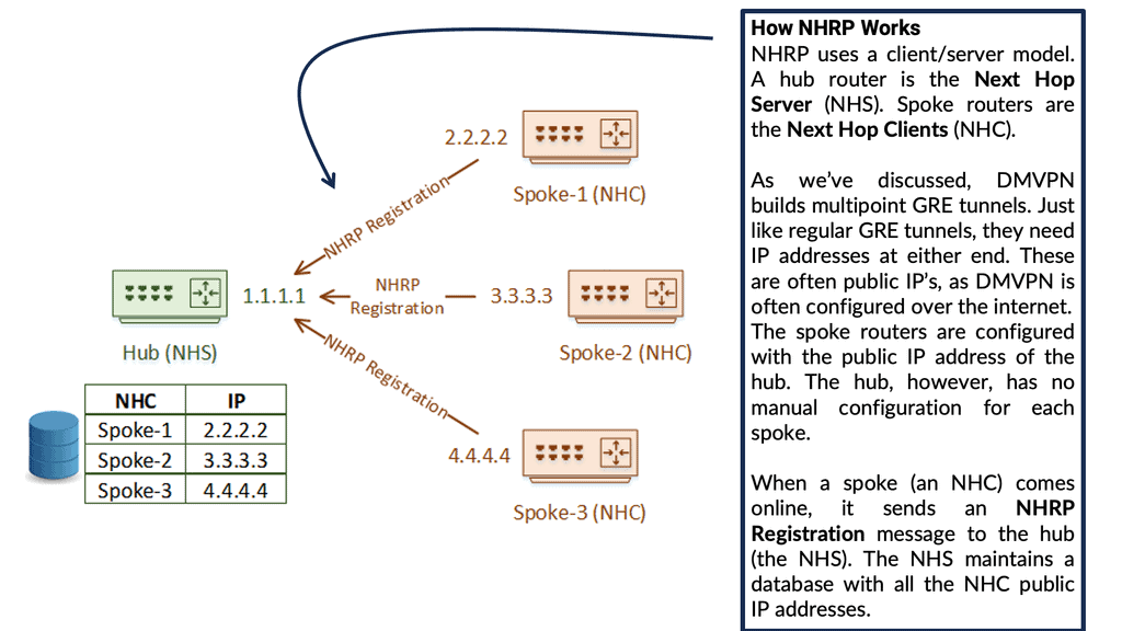
The NHRP can deploy spokes with assigned IP addresses, which can be connected from the central DMVPN hub. One branch router requires this protocol to find the public IP address of the second branch router. NHRP uses a “server-client” model, where one router functions as the NHRP server while the other routers are the NHRP clients. In the multipoint GRE/DMVPN topology, the hub router is the NHRP server, and all other routers are the spokes.
Each client registers with the server and reports its public IP address, which the server tracks in its cache. Then, through a process that involves registration and resolution requests from the client routers and resolution replies from the server router, traffic is enabled between various routers in the DMVPN.
4th Lab Guide: Displaying the DMVPN configuration
NHC and NHS Design
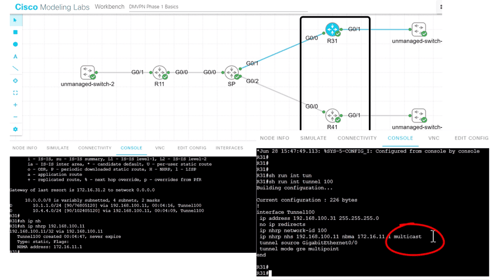
The following DMVPN configuration shows a couple of new topics. DMVPN works with an NHS and NHC design; the hub is the HHS. You can see this explicitly configured on the spokes, and this configuration needs to be on the spokes rather than the hubs.
The hub configuration is meant to be more dynamic. Also, if you recall, we are running EIGRP over the GRE tunnel. Two important points here. Firstly, we must consider a split-horizon as we have two spokes. Secondly, we need to use the “multicast” command.
Note:
- This is because EIGRP uses multicast HELLO messages to form neighbor relationships. If we had BGP running over the tunnel interface and not EIGRP, we would not need the multicast keywords. As BGP does not use multicast. The full command: IP nhrp nhs 192.168.100.11 nmba 172.16.11.1 multicast.
- On the spoke, we are telling the router that R11 is the NHS and to map its tunnel interface of 192.168.100.11 to the address 172.16.11.1 and to allow multicast traffic, or better explained, we are creating a new multicast mapping table.
5th Lab Guide: DMVPN over IPsec
Securing DMVPN
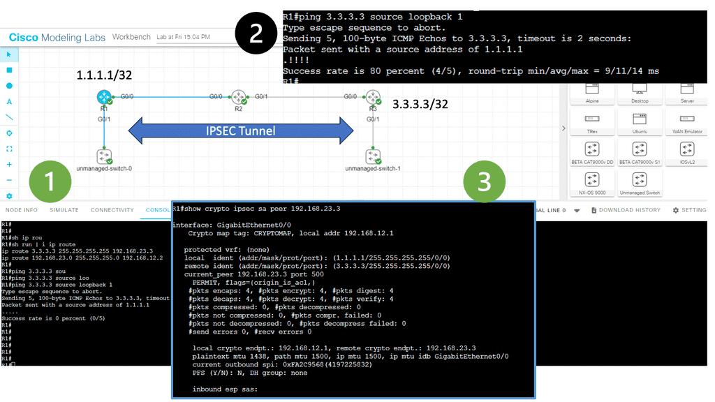
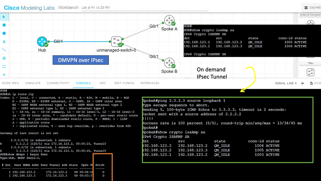
In the following screenshot, we have DMVPN operating over IPsec. So, I have connected the hub and two spokes into an unmanaged switch to simulate the WAN environment. A WAN and DMVPN do not have encryption by default. However, since you probably use DMVPN with the Internet as the underlying network, it might be wise to encrypt your tunnels.
In this network, we are running RIP v2 as the routing protocol. Remember that you must turn off the split horizon at the hub site. IPsec has phases 1 and 2 (don’t confuse them with the DMVPN phases). Firstly, we need an ISAKMP policy that matches all our routers. Then, for Phase 2, we require a transform set on each router that tells the router what encryption/hashing to use and if we want tunnel or transport mode.
Note:
- I used ESP with AES as the encryption algorithm for this configuration and SHA for hashing. The mode is essential; since we are using GRE, we have already used tunnels as a transport mode. If you use tunnel mode, we will have even more overhead, which is unnecessary.
- The primary test here was to run a ping between the spokes. Since the ping works behind the scenes, our two spoke routers will establish an IPsec tunnel. You can see the security association below:
IPsec Tunnels
An IPsec tunnel is a secure connection between two or more devices over an untrusted network using a set of cryptographic security protocols. The most common type of IPsec tunnel is the site-to-site tunnel, which connects two sites or networks. It allows two remote sites to communicate securely and exchange traffic between them. Another type of IPsec tunnel is the remote-access tunnel, which allows a remote user to connect to the corporate network securely.
When setting up an IPsec tunnel, several parameters, such as authentication method, encryption algorithm, and tunnel mode, must be configured. Depending on the organization’s needs, additional security protocols, such as Internet Key Exchange (IKE), can also be used for further authentication and encryption.
IPsec Tunnel Endpoint Discovery
Tunnel Endpoint Discovery (TED) allows routers to discover IPsec endpoints automatically so that static crypto maps must not be configured between individual IPsec tunnel endpoints. In addition, TED allows endpoints or peers to dynamically and proactively initiate the negotiation of IPsec tunnels to discover unknown peers.
These remote peers do not need to have TED configured to be discovered by inbound TED probes. So, while configuring TED, VPN devices that receive TED probes on interfaces — that are not configured for TED — can negotiate a dynamically initiated tunnel using TED.
DMVPN Checkpoint Main DMVPN Points To Consisder
|
DMVPN and Routing protocols
Routing protocols enable the DMVPN to find routes between different endpoints efficiently and effectively. Therefore, choosing the right routing protocol is essential to building a scalable and stable DMVPN. One option is to use Open Shortest Path First (OSPF) as the interior routing protocol. However, OSPF is best suited for small-scale DMVPN deployments.
The Enhanced Interior Gateway Routing Protocol (EIGRP) or Border Gateway Protocol (BGP) is more suitable for large-scale implementations. EIGRP is not restricted by the topology limitations of a link-state protocol and is easier to deploy and scale in a DMVPN topology. BGP can scale to many peers and routes, and it puts less strain on the routers compared to other routing protocols
DMVPN supports various routing protocols that enable efficient communication between network devices. In this section, we will explore three popular DMVPN routing protocols: Enhanced Interior Gateway Routing Protocol (EIGRP), Open Shortest Path First (OSPF), and Border Gateway Protocol (BGP). We will examine their characteristics, advantages, and use cases, allowing network administrators to make informed decisions when implementing DMVPN.
EIGRP: The Dynamic Routing Powerhouse
EIGRP is a distance vector routing protocol widely used in DMVPN deployments. This section will provide an in-depth look at EIGRP, discussing its features such as fast convergence, load balancing, and scalability. Furthermore, we will highlight best practices for configuring EIGRP in a DMVPN environment, optimizing network performance and reliability.
OSPF: Scalable and Flexible Routing
OSPF is a link-state routing protocol that offers excellent scalability and flexibility in DMVPN networks. This section will explore OSPF’s key attributes, including its hierarchical design, area types, and route summarization capabilities. We will also discuss considerations for deploying OSPF in a DMVPN environment, ensuring seamless connectivity and effective network management.
BGP: Extending DMVPN to the Internet
BGP, a path vector routing protocol, connects DMVPN networks to the global Internet. This section will focus on BGP’s unique characteristics, such as its autonomous system (AS) concept, policy-based routing, and route reflectors. We will also address the challenges and best practices of integrating BGP into DMVPN architectures.
6th Lab Guide: DMVPN Phase 1 and OSPF
DMVPN Routing
OSPF is not the best solution for DMVPN. Because it’s a link-state protocol, each spoke router must have the complete LSDB for the DMVPN area. Since we use a single subnet on the multipoint GRE interfaces, all spoke routers must be in the same area.
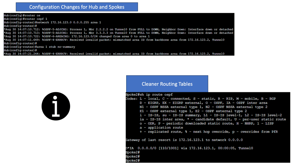
This is no problem with a few routers, but it doesn’t scale well when you have dozens or hundreds. Most spoke routers are probably low-end devices at branch offices that don’t like all the LSA flooding that OSPF might do within the area. One way to reduce the number of prefixes in the DMVPN network is to use a stub or total stub area.
Note:
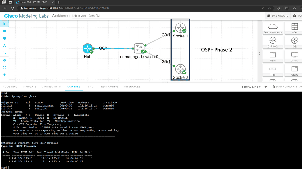
- The example below shows we are running OSPF between the Hub and the two spokes. OSPF network type can be viewed on the hub along with the status of DMVPN. Please take note of the next hop on the Spoke router when I do a show IP route OSPF.
- Each router has learned the networks on the different loopback interfaces. The next hop value is preserved when we use the broadcast network type.
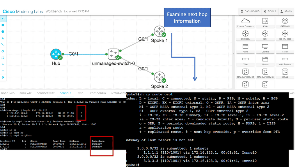
You have seen all the different OSPF Broadcast network types on DMVPN phase 1. As you can see, some stuff is in the routing tables. All traffic goes through the hub, so our spoke routers don’t need to know everything. Unfortunately, it’s impossible to summarize within the area. However, we can reduce the number of routes by changing the DMVPN area into a stub or total stub area.
Unlike the broadcast network type, point-to-point and point-to-multipoint network types do not preserve the spokes’ next-hop IP addresses.
7th Lab Guide: DMVPN Phase 2 with OSPF
DMVPN Routing
In the following example, we have DMVPN Phase 2 running with OSPF. We are using the Broadcast network type. However, the following OSPF network types are potentials for DMVPN phase 2.
- point-to-point
- broadcast
- non-broadcast
- point-to-multipoint
- point-to-multipoint non-broadcast
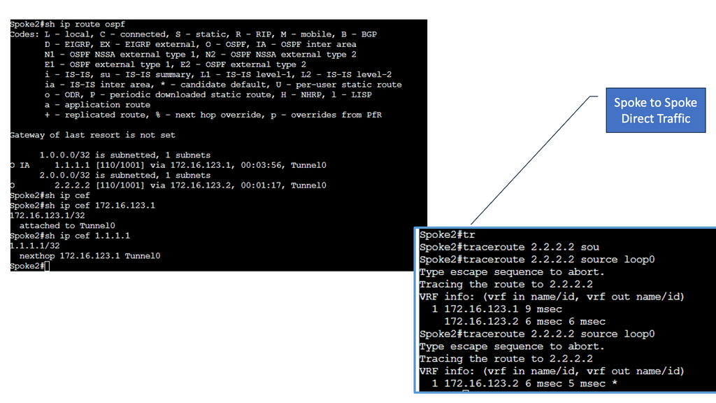
Below, all routers have learned the networks on each other’s loopback interfaces. Look closely at the next hop IP addresses for the 2.2.2.2/32 and 3.3.3.3/32 entries. This looks good; these are the IP addresses of the spoke routers. You can also see that 1.1.1.1/32 is an inter-area route. This is good; we can summarize networks “behind” the hub towards the spoke routers if we want to.
When running OSPF for DMVPN phase 2, you only have two choices if you want direct spoke-to-spoke communication: broadcast and non-broadcast. Let me give you an overview:
- Point-to-point: This will not work since we use multipoint GRE interfaces.
- Broadcast: This network type is your best choice. We are using it in the example above. The automatic neighbor discovery and correct next-hop addresses. Make sure that the spoke router can’t become DR or BDR. Here, we can use the priority commands and set them to 0 on the spokes.
- Non-broadcast: similar to broadcast, but you have to configure static neighbors.
- Point-to-multipoint: Don’t use this for DMVPN phase 2 since the hub changes the next hop address; you won’t have direct spoke-to-spoke communication.
- Point-to-multipoint non-broadcast: same story as point-to-multipoint, but you must also configure static neighbors.
DMVPN Deployment Scenarios:
Cisco DMVPN can be deployed in two ways:
- Hub-and-spoke deployment model
- Spoke-to-spoke deployment model
Hub-and-spoke deployment model: In this traditional topology, remote sites, which are the spokes, are aggregated into a headend VPN device. The headend VPN location would be at the corporate headquarters, known as the hub.
Traffic from any remote site to other remote sites would need to pass through the headend device. Cisco DMVPN supports dynamic routing, QoS, and IP Multicast while significantly reducing the configuration effort.
Spoke-to-spoke deployment model: Cisco DMVPN allows the creation of a full-mesh VPN, in which traditional hub-and-spoke connectivity is supplemented by dynamically created IPsec tunnels directly between the spokes.
With direct spoke-to-spoke tunnels, traffic between remote sites does not need to traverse the hub; this eliminates additional delays and conserves WAN bandwidth while improving performance.
Spoke-to-spoke capability is supported in a single-hub or multi-hub environment. Multihub deployments provide increased spoke-to-spoke resiliency and redundancy.
DMVPN Designs
The word phase is almost always connected to discussions on DMVPN design. DMVPN phase refers to the version of DMVPN implemented in a DMVPN design. As mentioned above, we can have two deployment models, each of which can be mapped to a DMVPN Phase.
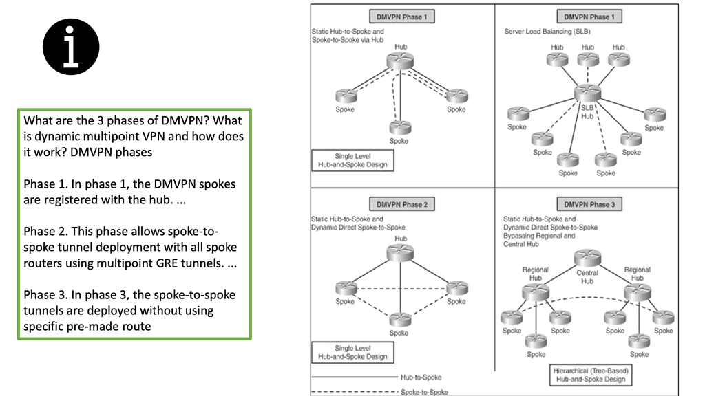
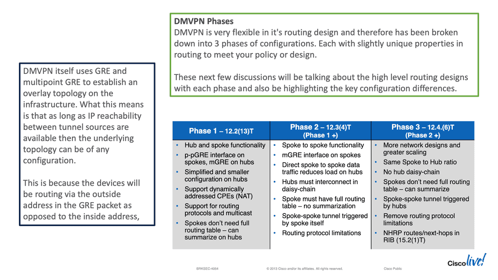
Cisco DMVPN as a solution was rolled out in different stages as the explanation became more widely adopted to address performance issues and additional improvised features. There are three main phases for DMVPN:
- Phase 1 – Hub-and-spoke
- Phase 2 – Spoke-initiated spoke-to-spoke tunnels
- Phase 3 – Hub-initiated spoke-to-spoke tunnels
The differences between the DMVPN phases are related to routing efficiency and the ability to create spoke-to-spoke tunnels. We started with DMVPN Phase 1, which only had a hub to spoke. This needed more scalability as we could not have direct spoke-to-spoke communication. Instead, the spokes could communicate with one another but were required to traverse the hub.
Then, we went to DMVPN Phase 2 to support spoke-to-spoke with dynamic tunnels. These tunnels were initially brought up by passing traffic via the hub. Later, Cisco developed DMVPN Phase 3, which optimized how spoke-to-spoke commutation happens and the tunnel build-up.
Dynamic multipoint virtual private networks began simply as what is best described as hub-and-spoke topologies. The primary tool for creating these VPNs combines Multipoint Generic Routing Encapsulation (mGRE) connections employed on the hub with traditional Point-to-Point (P2P) GRE tunnels on the spoke devices.
In this initial deployment methodology, known as a Phase 1 DMVPN, the spokes can only join the hub and communicate with one another through the hub. This phase does not use spoke-to-spoke tunnels. Instead, the spokes are configured for point-to-point GRE to the hub and register their logical IP with the non-broadcast multi-access (NBMA) address on the next hop server (NHS) hub.
It is essential to keep in mind that there is a total of three phases, and each one can influence the following:
- Spoke-to-spoke traffic patterns
- Routing protocol design
- Scalability
DMVPN Design Options
The disadvantage of a single hub router is that it’s a single point of failure. Once your hub router fails, the entire DMVPN network is gone.
We need another hub router to add redundancy to our DMVPN network. There are two options for this:
- Dual hub – Single Cloud
- Dual hub – Dual Cloud
With the single cloud option, we use a single DMVPN network but add a second hub. The spoke routers will use only one multipoint GRE interface, and we configure the second hub as a next-hop server. The dual cloud option also has two hubs, but we will use two DMVPN networks, meaning all spoke routers will get a second multipoint GRE interface.
Understanding DMVPN Dual Hub Single Cloud:
DMVPN dual hub single cloud is a network architecture that provides redundancy and high availability by utilizing two hub devices connected to a single cloud. The cloud can be an internet-based infrastructure or a private WAN. This configuration ensures the network remains operational even if one hub fails, as the other hub takes over the traffic routing responsibilities.
Benefits of DMVPN Dual Hub Single Cloud:
1. Redundancy: With dual hubs, organizations can ensure network availability even during hub device failures. This redundancy minimizes downtime and maximizes productivity.
2. Load Balancing: DMVPN dual hub single cloud allows for efficient load balancing between the two hubs. Traffic can be distributed evenly, optimizing bandwidth utilization and enhancing network performance.
3. Scalability: The architecture is highly scalable, allowing organizations to easily add new sites without reconfiguring the entire network. New sites can be connected to either hub, providing flexibility and ease of expansion.
4. Simplified Management: DMVPN dual hub single cloud simplifies network management by centralizing control and reducing the complexity of VPN configurations. Changes and updates can be made at the hub level, ensuring consistent policies across all connected sites.
The disadvantage is that we have limited control over routing. Since we use a single multipoint GRE interface, making the spoke routers prefer one hub over another is challenging.
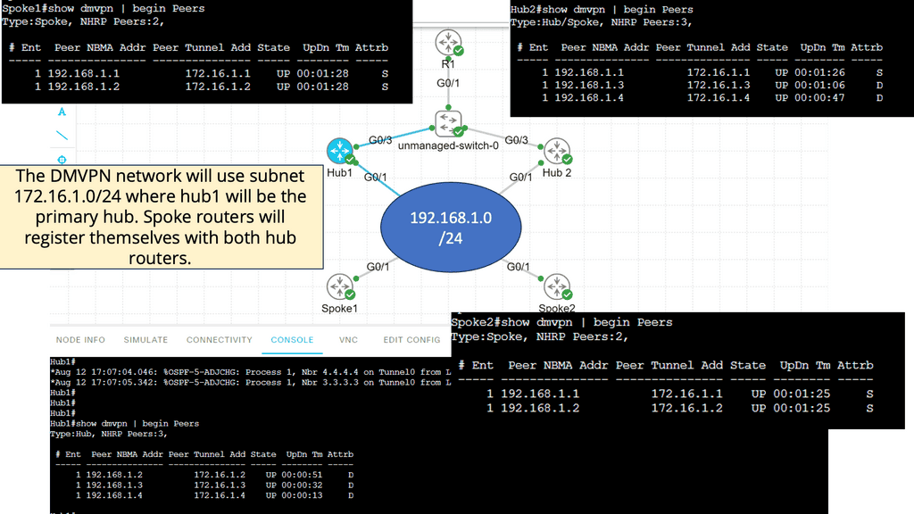
8th Lab Guide: DMVPN Dual Hub Single Cloud
DMVPN Advanced Configuration
Below is a DMVPN network with two hubs and two spoke routers. Hub1 will be the primary hub, and hub2 will be the secondary hub. We use a single DMVPN network; each router only has one multipoint GRE interface. On top of that, we have R1 on the leading site where we use the 10.10.10.0/24 subnet. Behind R1, we have a loopback interface with IP address 1.1.1.1/32.
Note:
- The two hub routers and spoke routers are connected to the Internet. Usually, you would connect the two hub routers to different ISPs. To keep it simple, I combined all routers into the 192.168.1.0/24 subnet, represented as an unmanaged switch in the lab below.
- Each spoke router has a loopback interface with an IP address. The DMVPN network will use subnet 172.16.1.0/24, where hub1 will be the primary hub. Spoke routers will register themselves with both hub routers.
Summary of DMVPN Phases
Phase 1—Hub-to-Spoke Designs: Phase 1 was the first design introduced for hub-to-spoke implementation, where spoke-to-spoke traffic would traverse via the hub. Phase 1 also introduced daisy chaining of identical hubs for scaling the network, thereby providing Server Load Balancing (SLB) capability to increase the CPU power.
Phase 2—Spoke-to-Spoke Designs: Phase 2 design introduced the ability for dynamic spoke-to-spoke tunnels without traffic going through the hub, intersite communication bypassing the hub, thereby providing greater scalability and better traffic control.
In Phase 2 network design, each DMVPN network is independent of other DMVPN networks, causing spoke-to-spoke traffic from different regions to traverse the regional hubs without going through the central hub.
Phase 3—Hierarchical (Tree-Based) Designs: Phase 3 extended Phase 2 design with the capability to establish dynamic and direct spoke-to-spoke tunnels from different DMVPN networks across multiple regions. In Phase 3, all regional DMVPN networks are bound to form a single hierarchical (tree-based) DMVPN network, including the central hubs.
As a result, spoke-to-spoke traffic from different regions can establish direct tunnels with each other, thereby bypassing both the regional and main hubs.
DMVPN Architecture |
|
DMVPN Design recommendation
Which deployment model can you use? The 80:20 traffic rule can be used to determine which model to use:
- If 80 percent or more of the traffic from the spokes is directed into the hub network itself, deploy the hub-and-spoke model.
- Consider the spoke-to-spoke model if more than 20 percent of the traffic is meant for other spokes.
The hub-and-spoke model is usually preferred for networks with a high volume of IP Multicast traffic.
Architecture
Medium-sized and large-scale site-to-site VPN deployments require support for advanced IP network services such as:
● IP Multicast: Required for efficient and scalable one-to-many (i.e., Internet broadcast) and many-to-many (i.e., conferencing) communications and commonly needed by voice, video, and specific data applications
● Dynamic routing protocols: Typically required in all but the smallest deployments or wherever static routing is not manageable or optimal
● QoS: Mandatory to ensure performance and quality of voice, video, and real-time data applications
Traditionally, supporting these services required tunneling IPsec inside protocols such as Generic Route Encapsulation (GRE), which introduced an overlay network, making it complex to set up and manage and limiting the solution’s scalability.
Indeed, traditional IPsec only supports IP Unicast, making deploying applications that involve one-to-many and many-to-many communications inefficient. Cisco DMVPN combines GRE tunneling and IPsec encryption with Next-Hop Resolution Protocol (NHRP) routing to meet these requirements while reducing the administrative burden.
How DMVPN Works |
|
How DMVPN Works
DMVPN builds a dynamic tunnel overlay network.
• Initially, each spoke establishes a permanent IPsec tunnel to the hub. (At this stage, spokes do not establish tunnels with other spokes within the network.) The hub address should be static and known by all of the spokes.
• Each spoke registers its actual address as a client to the NHRP server on the hub. The NHRP server maintains an NHRP database of the public interface addresses for each spoke.
• When a spoke requires that packets be sent to a destination (private) subnet on another spoke, it queries the NHRP server for the real (outside) addresses of the other spoke’s destination to build direct tunnels.
• The NHRP server looks up the NHRP database for the corresponding destination spoke and replies with the real address for the target router. NHRP prevents dynamic routing protocols from discovering the route to the correct spoke. (Dynamic routing adjacencies are established only from spoke to the hub.)
• After the originating spoke learns the peer address of the target spoke, it initiates a dynamic IPsec tunnel to the target spoke.
• Integrating the multipoint GRE (mGRE) interface, NHRP, and IPsec establishes a direct dynamic spoke-to-spoke tunnel over the DMVPN network.
The spoke-to-spoke tunnels are established on demand whenever traffic is sent between the spokes. After that, packets can bypass the hub and use the spoke-to-spoke tunnel directly.
Feature Design of Dynamic Multipoint VPN
The Dynamic Multipoint VPN (DMVPN) feature combines GRE tunnels, IPsec encryption, and NHRP routing to provide users with ease of configuration via crypto profiles—which override the requirement for defining static crypto maps—and dynamic discovery of tunnel endpoints.
This feature relies on the following two Cisco-enhanced standard technologies:
- NHRP is a client-server protocol where the hub is the server and the spokes are the clients. The hub maintains an NHRP database of each spoke’s public interface addresses. Each spoke registers its real address when it boots and queries the NHRP database for the real addresses of the destination spokes to build direct tunnels.
- mGRE Tunnel Interface –Allows a single GRE interface to support multiple IPsec tunnels and simplifies the size and complexity of the configuration.
- Each spoke has a permanent IPsec tunnel to the hub, not to the other spokes within the network. Each spoke registers as a client of the NHRP server.
- When a spoke needs to send a packet to a destination (private) subnet on another spoke, it queries the NHRP server for the real (outside) address of the destination (target) spoke.
- After the originating spoke “learns” the peer address of the target spoke, a dynamic IPsec tunnel can be initiated into the target spoke.
- The spoke-to-spoke tunnel is built over the multipoint GRE interface.
- The spoke-to-spoke links are established on demand whenever there is traffic between the spokes. After that, packets can bypass the hub and use the spoke-to-spoke tunnel.
Cisco DMVPN Solution Architecture
DMVPN allows IPsec VPN networks to scale hub-to-spoke and spoke-to-spoke designs better, optimizing performance and reducing communication latency between sites.
DMVPN offers a wide range of benefits, including the following:
• The capability to build dynamic hub-to-spoke and spoke-to-spoke IPsec tunnels
• Optimized network performance
• Reduced latency for real-time applications
• Reduced router configuration on the hub that provides the capability to dynamically add multiple spoke tunnels without touching the hub configuration
• Automatic triggering of IPsec encryption by GRE tunnel source and destination, assuring zero packet loss
• Support for spoke routers with dynamic physical interface IP addresses (for example, DSL and cable connections)
• The capability to establish dynamic and direct spoke-to-spoke IPsec tunnels for communication between sites without having the traffic go through the hub; that is, intersite communication bypassing the hub
• Support for dynamic routing protocols running over the DMVPN tunnels
• Support for multicast traffic from hub to spokes
• Support for VPN Routing and Forwarding (VRF) integration extended in multiprotocol label switching (MPLS) networks
• Self-healing capability maximizing VPN tunnel uptime by rerouting around network link failures
• Load-balancing capability offering increased performance by transparently terminating VPN connections to multiple headend VPN devices
Network availability over a secure channel is critical in designing scalable IPsec VPN solutions prepared with networks becoming geographically distributed. DMVPN solution architecture is by far the most effective and scalable solution available.