IP Forwarding
What is IP forwarding?
IP forwarding, or packet forwarding, is a fundamental function of network routers. It involves directing data packets from one network interface to another, ultimately reaching their intended destination. This intelligent routing mechanism plays a crucial role in ensuring efficient data transmission across networks, enabling seamless communication.
How Does IP Forwarding Work?
Underneath the surface, IP forwarding operates based on the principles of routing tables. These tables contain valuable network information, including IP addresses, subnet masks, and next-hop destinations. When a data packet arrives at a router, it examines the destination IP address and consults its routing table to determine the appropriate interface to forward the packet. This dynamic decision-making process allows routers to navigate through the vast realm of interconnected networks efficiently.
The Role of Routing Tables
Routing tables are vital to the IP forwarding process. They contain information about the various network paths available, including the next hop and metrics that define the path’s efficiency. Routers constantly update their routing tables using protocols like OSPF (Open Shortest Path First) and BGP (Border Gateway Protocol) to adapt to changes in the network topology. This dynamic updating process allows the network to maintain optimal performance even as conditions change.
Common Scenarios for IP Forwarding
IP forwarding is ubiquitous in various networking scenarios. For example, in a corporate environment, IP forwarding enables communication between different departments by routing data through the company’s internal network. In the wider internet, IP forwarding allows data to traverse multiple networks, hopping from one router to another until it reaches its destination. Understanding these scenarios can help network administrators design efficient and reliable networks.
Troubleshooting IP Forwarding Issues
Network issues related to IP forwarding can be challenging to diagnose and resolve. Common problems include misconfigured routing tables, outdated firmware, and physical connectivity issues. Network administrators often use tools like traceroute and ping to test the path and latency of data packets, helping them identify where issues may be occurring. Regular monitoring and maintenance of routing tables and network infrastructure are crucial to preventing and addressing these issues.
Recap: Identifying Networks
To troubleshoot the network effectively, you can use a range of tools. Some are built into the operating system, while others must be downloaded and run. Depending on your experience, you may choose a top-down or a bottom-up approach.
IP Forwarding Algorithms and Protocols
Various algorithms and protocols optimize the routing process. Some popular algorithms include shortest-path algorithms like Dijkstra’s and Bellman-Ford. Additionally, protocols such as Open Shortest Path First (OSPF) and Border Gateway Protocol (BGP) are widely used in IP forwarding to establish and maintain efficient routing paths.
**IP forwarding is required to use the system as a router**
– Imagine a server with two physical Ethernet ports connected to two different networks (your internal network and the outside world via a DSL modem). The system can communicate on either network if you connect and configure those two interfaces. Packets from one network cannot reach another due to the lack of forwarding. Let’s look at ‘route add’ as an example.
– If you have two network interfaces, you must add two routes, one for each interface. When determining where to send network packets, kernels choose the most suitable route. The kernel does not check the origin of packets when forwarding is disabled. The kernel discards any packet that comes from a different interface.
There is no need to have two physical network interfaces when using a router. VLAN-based servers, for instance, can transfer IP packets between VLANs, but they only have one physical network interface. It is known as a one-armed router. IP forwarding is unnecessary if you have only one physical network interface. IP forwarding must be enabled to transfer packets between two network interfaces (real or virtual) on the same network. Transferring packets between the interfaces makes little sense since they are already on the same network.
Understanding Routing
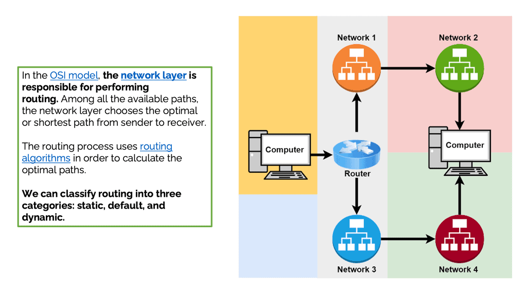
– In the OSI model, the network layer is responsible for routing. Among all the available paths, the network layer chooses the optimal or shortest path from sender to receiver. The routing process uses routing algorithms to calculate the optimal paths.
– We can classify routing into three categories: static, default, and dynamic. Static routing is a nonadaptive type in which the administrator adds and defines the route the data needs to follow to reach the destination from the source. In default routing, all packets take a predefined default path. It’s helpful in bulk data transmission and networks with a single exit point. Finally, dynamic routing, also known as adaptive routing, uses dynamic protocols to find new routes to reach the receiver.
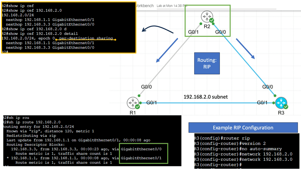
– Routing is like the GPS of a network, determining the best path for data packets to travel from one network to another. It involves exchanging information between routers, enabling them to make intelligent decisions about forwarding data. Routing protocols, such as OSPF or BGP, allow routers to communicate and build routing tables, ensuring efficient and reliable data transmission across networks. While OSPF and BGP are better for production networks, RIP can be used in a lab environment to demonstrate how dynamic routing protocols work.
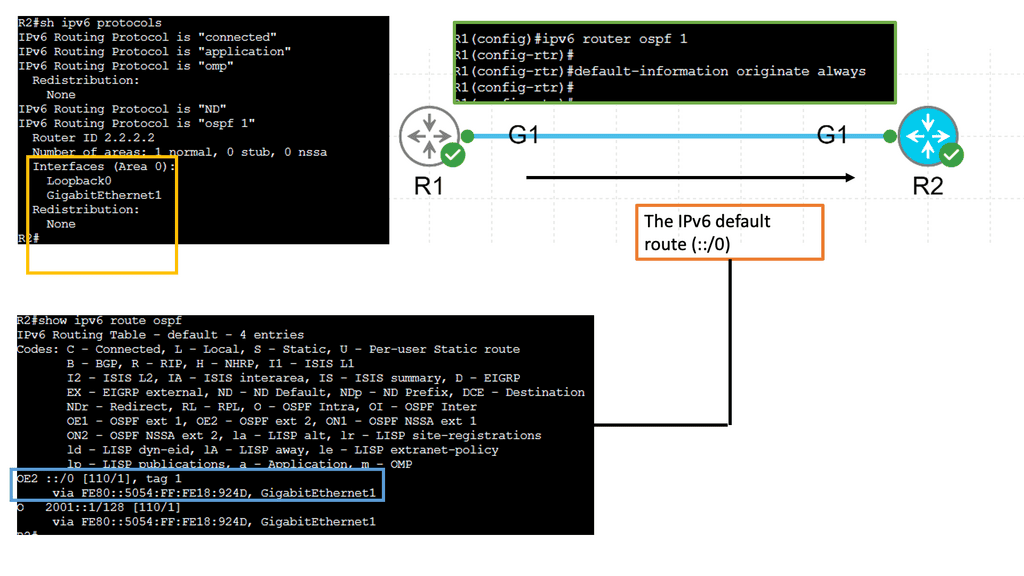
Example: OSPFv3
Understanding OSPFv3
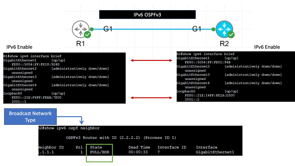
OSPFv3, or Open Shortest Path First version 3, is an enhanced version of OSPF designed specifically for IPv6 networks. It serves as a link-state routing protocol, allowing routers to dynamically exchange routing information and calculate the most efficient paths for data transmission. Unlike its predecessor, OSPFv3 is not backward compatible with IPv4, making it a dedicated routing protocol for IPv6 networks.
OSPFv3 has several notable features that make it a preferred choice for network administrators. First, it supports IPv6 addressing, enabling seamless integration and efficient routing in modern networks. Second, OSPFv3 introduces improved security mechanisms, including using IPsec, which ensures secure communication between routers. Third, It offers better scalability, faster convergence, and extensive support for multiple routing domains.
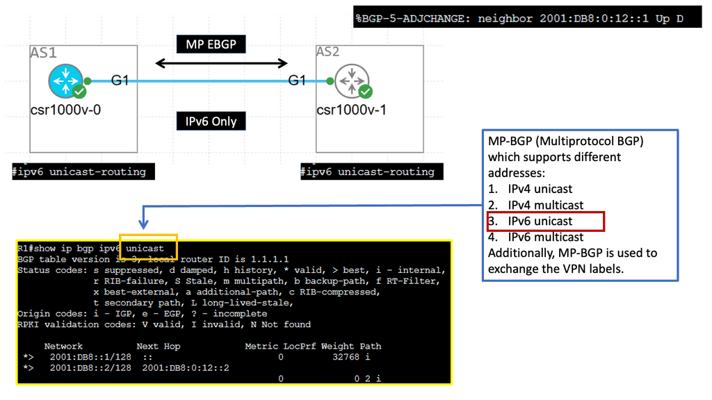
Example: MP BGP with IPv6 Prefix
Understanding MP-BGP
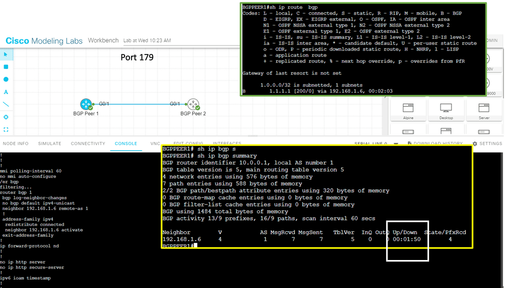
MP-BGP, a Border Gateway Protocol (BGP) variant, is designed to support multiple address families and protocols. It enables the exchange of routing information across different networks, making it a powerful tool for network administrators. With the emergence of IPv6, MP-BGP has become even more critical in facilitating seamless communication in the new era of internet connectivity.
IPv6, the successor to IPv4, brings many advantages including a larger address space, improved security, and enhanced end-to-end connectivity. By incorporating IPv6 adjacency into MP-BGP, network operators can harness the full potential of IPv6 in their routing infrastructure. This allows for efficient routing of IPv6 traffic and enables seamless integration with existing IPv4 networks.
Unraveling Switching
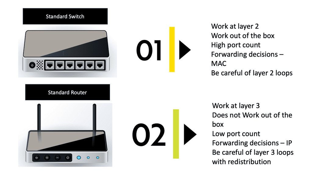
Switches are essential to a network’s functioning. They connect computers, wireless access points, printers, servers, and printers within a building or campus, allowing devices to share information and communicate. Plug-and-play network switches do not require configuration and are designed to work immediately. Unmanaged switches provide basic connectivity. They are often found in home networks or places where more ports are needed, such as your desk, lab, or conference room.
A managed switch offers higher security and features because it can be configured according to your network. Through greater control, your network can be better protected, and the quality of service for users can be improved. Switching, however, focuses on efficiently delivering data packets within a network. Switches operate at the data link layer of the OSI model and use MAC addresses to direct packets to their intended destinations.
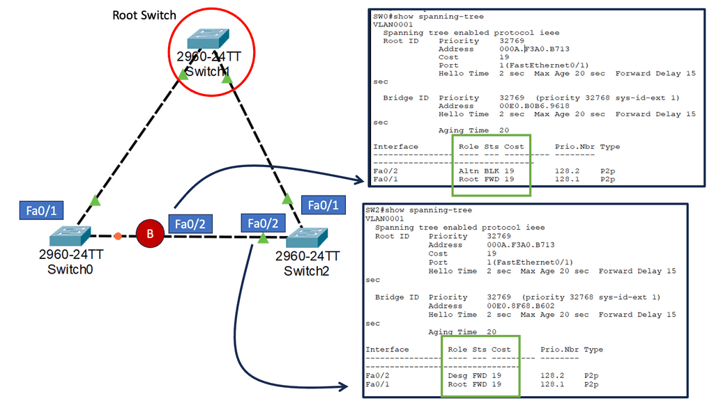
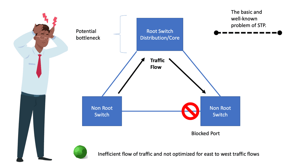
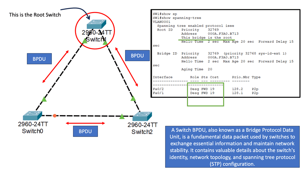
By building and maintaining MAC address tables, switches facilitate fast and accurate data forwarding within local networks. Spanning Tree Protocol (STP) identifies redundant links and shuts them down to prevent possible network loops. To determine the root bridge, all switches in the network exchange BPDU messages.
Comparing Routing and Switching
While routing and switching contribute to a network’s functioning, they differ in scope and operation. Routing occurs at the network layer (Layer 3) and is responsible for interconnecting networks, enabling communication between different subnets or autonomous systems. Switching, on the other hand, operates at the data link layer (Layer 2) and focuses on efficient data delivery within a local network. The two most essential equipment for building a small office network are switches and routers. Both devices perform different functions within a network despite their similar appearances.
Switches: what are they?
In a small business network, switches facilitate the sharing of resources by connecting computers, printers, and servers. Whether these connected devices are in a building or on a campus, they can share information and talk to each other thanks to the switch. Switches tie devices together, making it impossible to build a small business network without them.
What is a router?
Routers connect multiple switches and their respective networks to form an even more extensive network, like switches connecting various devices. One or more of these networks may be at one location. When setting up a small business network, you will need one or more routers. Networked devices and multiple users can access the Internet through the router and connect to various networks.
A router acts as a dispatcher, directing traffic and selecting the best route for data packets to travel across the network. With a router, your business can connect to the world, protect information from security threats, and prioritize devices.
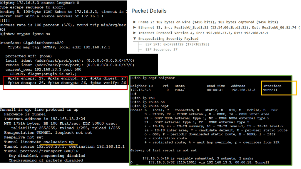
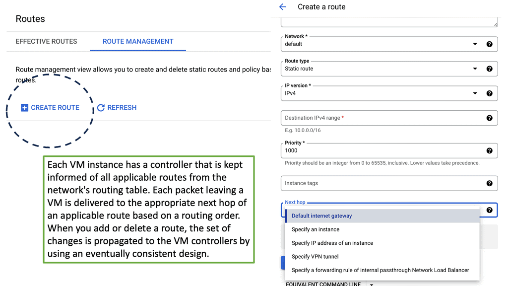
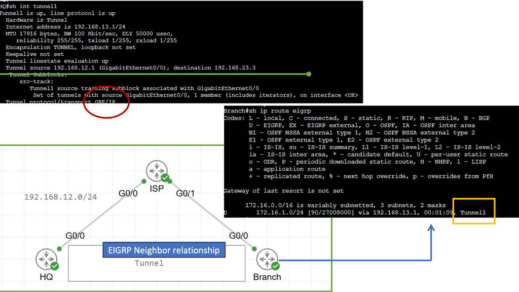
In the context of routing, the next hop refers to the next network device or hop to which a packet should be forwarded to reach its destination. It represents the immediate next step in the data’s journey through the network and determines the network interface or IP address to which the packet should be sent. Regarding tunneling protocols, the next hop can be the tunnel interface.
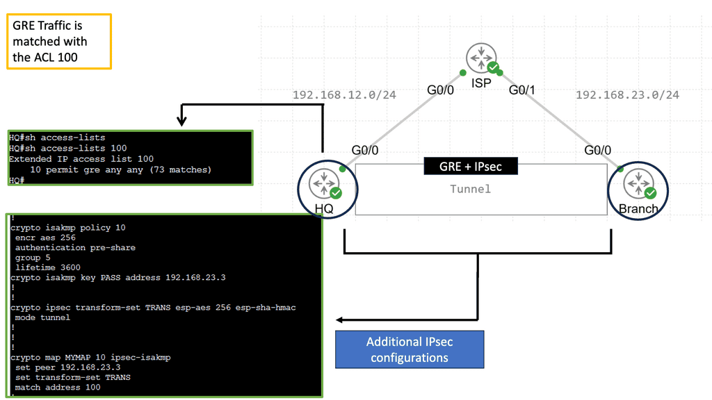
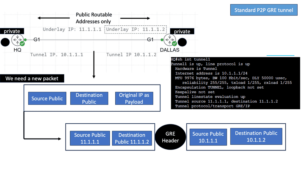
Example Technology: GRE Tunneling
Before diving into the intricacies of GRE tunneling, it is crucial to grasp its fundamental concepts. GRE tunneling involves encapsulating one protocol within another, typically encapsulating IP packets within IP packets. This encapsulation creates a virtual tunnel to transmit data between two networks securely. Routing the encapsulated packets through the tunnel allows network administrators to establish seamless connectivity between geographically separated networks, regardless of the underlying network infrastructure.
 Implementation of GRE Tunnels
Implementing GRE tunnels requires a systematic approach to ensure their successful deployment. Firstly, it is essential to identify the source and destination networks between which the tunnel will be created. Once identified, the next step involves configuring the tunnel interfaces on the corresponding devices.
This includes specifying the tunnel source and destination IP addresses and selecting suitable tunneling protocols and parameters. Appropriate routing configurations must also be applied to ensure traffic flows correctly through the tunnel. Properly implementing GRE tunnels lays the foundation for efficient and secure network communication.
What are Routing Algorithms?
Routing algorithms are computational procedures routers use to determine the optimal path for data packets to travel from the source to the destination in a network. They are crucial in ensuring efficient and effective data transmission, minimizing delays and congestion, and improving network performance. Routing algorithms employ hop count, bandwidth, delay, and load metrics to determine the optimal path for data packets. These algorithms rely on routing tables, which store information about available routes and their associated metrics. By evaluating these metrics, routers make informed decisions to forward packets along the most suitable path to reach the destination.
Distance vector routing
Distance vector routing protocols allow routers to advertise routing information to neighbors from their perspective, modified from the original route. As a result, distance vector protocols do not have an exact map of the entire network; instead, their database reflects how a neighbor router can reach the destination network and its distance from it. Other routers may be on their path toward those networks, but I do not know how many. In addition to requiring less CPU and memory, distance vector protocols can be run on low-end routers.
For example, distance vector protocols are often compared to road signs at intersections that indicate the destination is 20 miles away; people blindly follow these signs without realizing if there is a shorter or better route to the destination or whether the sign is even accurate.
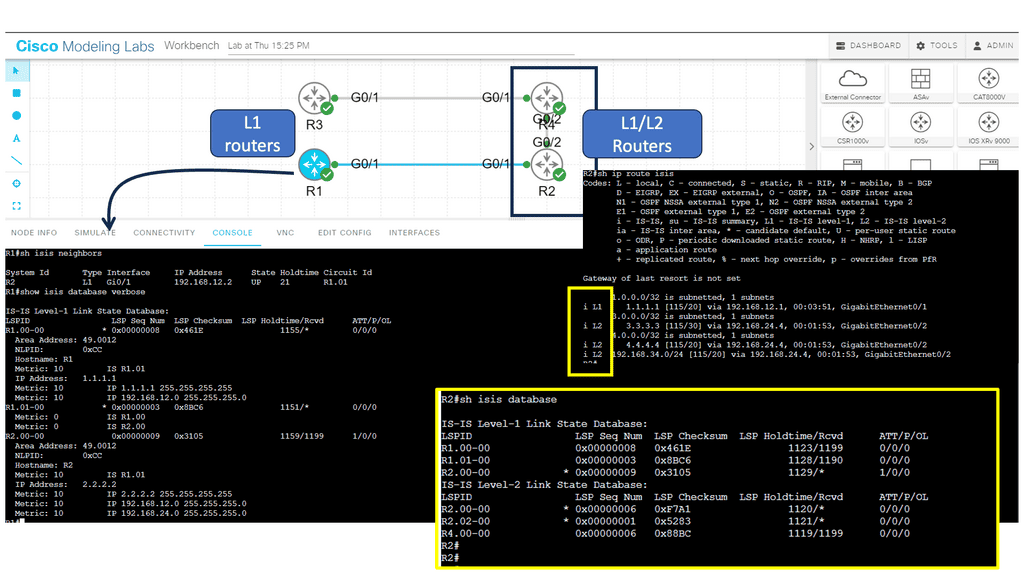
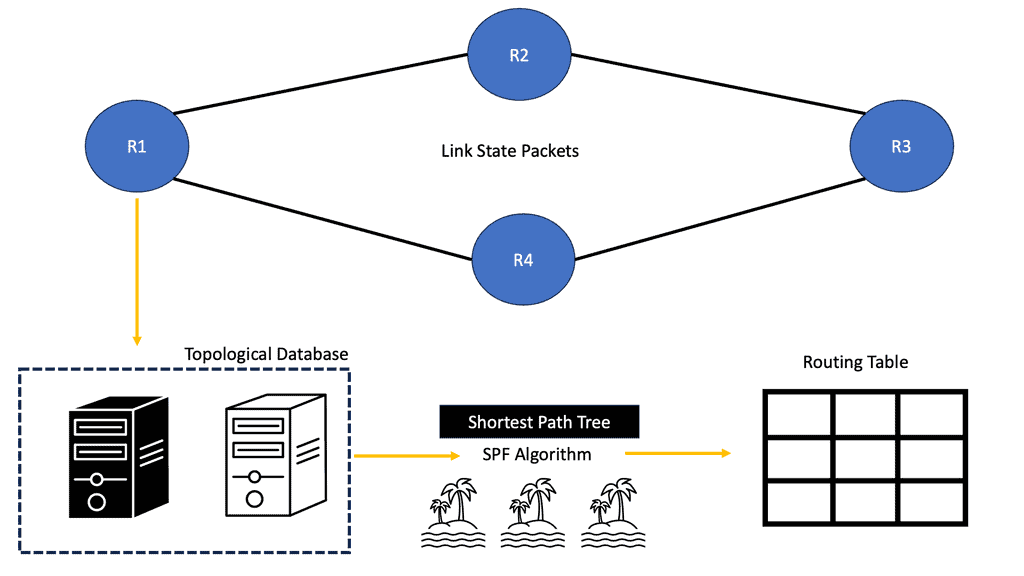
Link-State Algorithms
Each connected and directly connected router advertises the link state and metric in link-state dynamic IP routing protocols. Enterprise and service provider networks commonly use OSPF and IS-IS link-state routing protocols. IS-IS advertisements are called link-state packets (LSPs), while OSPF advertisements are called link-state advertisements (LSAs).
Whenever a router receives an advertisement from a neighbor, it stores the information in a local link-state database (LSDB) and advertises it to all its neighbors. As advertised by the originating router, link-state information is essentially flooded throughout the network unchanged. A synchronized and identical map of the network is provided to all routers in the network.
Routing neighbor relationship
Routing neighbor relationships refer to the connections between neighboring network routers. These relationships facilitate the exchange of routing information, allowing routers to communicate and make informed forwarding decisions efficiently. Routers can build a dynamic and adaptive network topology by forming these relationships.
Once established, routing neighbor relationships require ongoing maintenance to ensure stability and reliability. Routers periodically exchange keep-alive messages to confirm their neighbors’ continued presence. Additionally, routers monitor their neighbors’ health and reachability through various mechanisms, such as dead interval timers and neighbor state tracking.
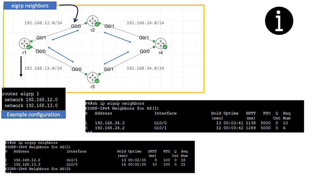
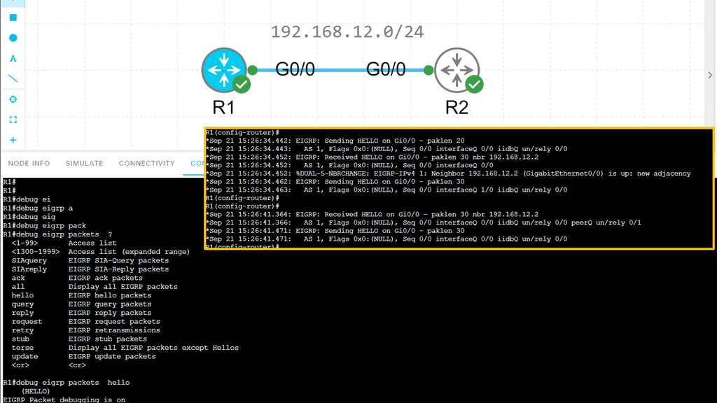
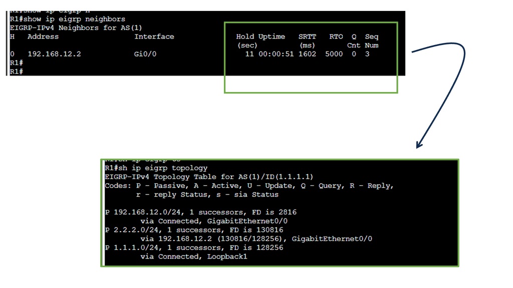
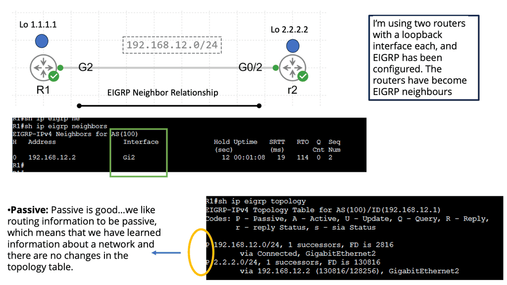
Example: EIGRP neighbor relationship
The Hello Protocol is the cornerstone of EIGRP neighbor relationship formation. Routers using EIGRP send Hello packets to discover and establish neighbors. These packets contain information such as router ID, hold time and other parameters. By exchanging Hello packets, routers can identify potential neighbors and establish a neighbor relationship.
Once hello packets are exchanged, routers engage in neighbor discovery and verification. During this phase, routers compare the received Hello packet information with their configured parameters. If the information matches, a neighbor relationship is formed. This verification step ensures that only compatible routers become neighbors, enhancing the network’s stability and reliability.
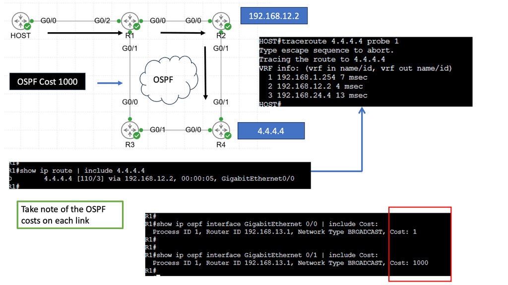
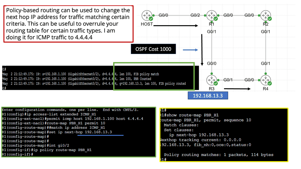
Understanding Policy-Based Routing
Policy-based routing, also known as PBR, is a technique that allows network administrators to make routing decisions based on specific policies or conditions. Traditional routing relies solely on destination IP addresses, whereas PBR considers additional factors such as source IP addresses, protocols, or packet attributes. By leveraging these conditions, network administrators can exert fine-grained control over traffic flow.
The flexibility offered by policy-based routing brings numerous advantages. First, it enables the implementation of customized routing policies tailored to specific requirements. Whether prioritizing real-time applications or load balancing across multiple links, PBR empowers administrators to optimize network performance based on their unique needs. Policy-based routing enhances network security by allowing traffic to be redirected through firewalls or VPNs, providing an added layer of protection.
Implementing Policy-Based Routing
Implementing policy-based routing involves several key steps. The first step is defining the routing policy, which consists in determining the conditions and actions to take. This can be done through access control lists (ACLs) or route maps. Once the policy is defined, it must be applied to the desired interfaces or traffic flows. Testing and monitoring the policy’s effectiveness is crucial to ensure that desired outcomes are achieved.
**PBR vs. IP Forwarding**
Understanding IP Forwarding
IP forwarding is a fundamental concept in networking. It involves forwarding data packets between network interfaces based on their destination IP addresses. IP forwarding operates at the network layer of the OSI model and is essential for routing packets across multiple networks. It relies on routing tables to determine the best path for packet transmission.
Unveiling Policy-Based Routing (PBR)
Policy-based routing goes beyond traditional IP forwarding by allowing network administrators to control the path of packets based on specific policies or criteria. These policies can include source IP address, destination IP address, protocols, or port numbers. PBR enables granular control over network traffic, making it a powerful tool for shaping traffic flows within a network.
Traffic Engineering and Load Balancing: PBR excels in scenarios where traffic engineering and load balancing are crucial. By selectively routing packets based on specific policies, network administrators can distribute traffic across multiple paths, optimizing bandwidth utilization and avoiding congestion. On the other hand, IP forwarding lacks the flexibility to dynamically manage traffic flows, making it less suitable for such use cases.
Security and Access Control: PBR offers an advantage when enforcing security measures and access control. Network administrators can steer traffic through firewalls, intrusion detection systems, or other security devices by defining policies based on source IP addresses or protocols. IP forwarding cannot selectively route traffic based on such policies, limiting its effectiveness in security-focused environments.
MPLS Forwarding
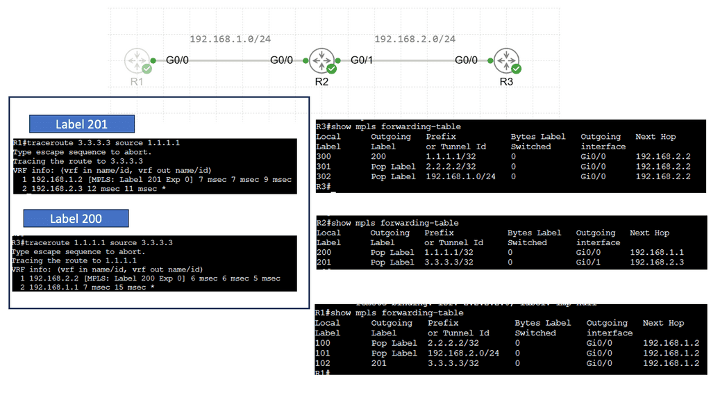
MPLS, short for Multiprotocol Label Switching, is used in telecommunications networks to efficiently direct data packets. Unlike traditional IP routing, MPLS employs labels to guide packets along predetermined paths, known as Label Switched Paths (LSPs). These labels are attached to the packets, allowing routers to forward them based on this labeling, significantly improving network performance.
Within an MPLS network, routers use labels to determine the optimal path for data packets. Each router along the LSP has a forwarding table that maps incoming labels to outgoing interfaces. Routers swap labels as packets traverse the network, ensuring proper forwarding based on predetermined policies and traffic engineering considerations.
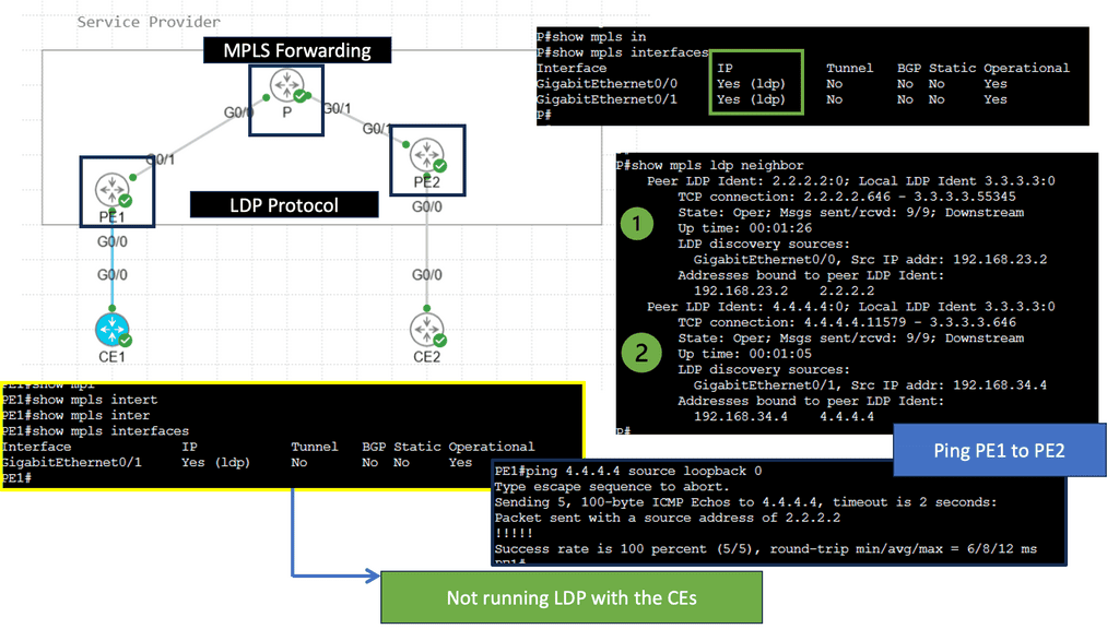
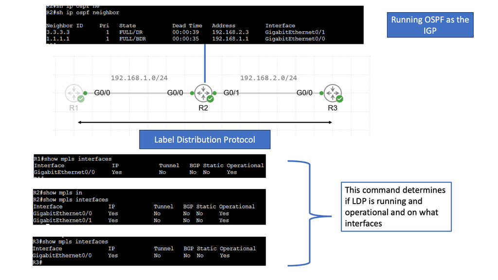
Understanding MPLS LDP
MPLS LDP is a protocol used in MPLS networks to distribute labels, facilitating efficient packet forwarding. It establishes label-switched paths (LSPs) and enables routers to make forwarding decisions based on labels rather than traditional IP routing. By understanding the fundamentals of MPLS LDP, we can unlock the potential of this powerful technology.
MPLS LDP brings several benefits to network operators. Firstly, it allows for traffic engineering, enabling precise control over how packets are routed through the network. This enhances performance and optimizes resource utilization. Additionally, MPLS LDP provides fast convergence and scalability, making it ideal for large-scale networks. Its label-based forwarding mechanism also facilitates traffic isolation and improves security.
**MPLS Forwarding vs IP Forwarding**
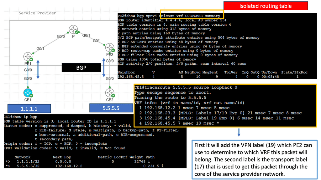
MPLS (Multi-Protocol Label Switching) is a flexible and efficient forwarding mechanism in modern networks. At its core, MPLS forwarding relies on label-switching to expedite data transmission. It operates at the network layer (Layer 3) and involves the encapsulation of packets with labels. These labels contain crucial routing information, allowing faster and more deterministic forwarding decisions. MPLS forwarding is widely adopted in service provider networks to enhance traffic engineering, quality of service (QoS), and virtual private networks (VPNs) capabilities.
On the other hand, IP (Internet Protocol) forwarding is the traditional method of routing packets across networks. It is based on the destination IP address present in the packet header. IP forwarding operates at the network layer (Layer 3) and is the backbone of the internet, responsible for delivering packets from the source to the destination. Unlike MPLS forwarding, IP forwarding does not involve encapsulating packets with labels.
Key Differences
While MPLS and IP forwarding share the objective of routing packets, several key differences set them apart. Firstly, MPLS forwarding introduces an additional layer of encapsulation with labels, allowing for more efficient and deterministic routing decisions. In contrast, IP forwarding relies solely on the destination IP address. Secondly, MPLS forwarding provides enhanced traffic engineering capabilities, enabling service providers to optimize network resource utilization and prioritize certain types of traffic. IP forwarding, being more straightforward, does not possess these advanced traffic engineering features.
Benefits of MPLS Forwarding
MPLS forwarding offers several advantages in networking. First, it provides improved scalability, as the label-switching mechanism allows for more efficient handling of large traffic volumes. Second, MPLS forwarding enables the implementation of QoS mechanisms, ensuring critical applications receive the necessary bandwidth and prioritization. Additionally, MPLS forwarding facilitates the creation of secure and isolated VPNs, offering enhanced privacy and connectivity options.
Benefits of IP Forwarding
While MPLS forwarding has its advantages, IP forwarding remains a reliable and widely used forwarding technique. It is simpler to implement and manage, making it suitable for smaller networks or scenarios without advanced traffic engineering features. Moreover, IP forwarding is the foundation of the Internet, making it universally compatible and widely supported.
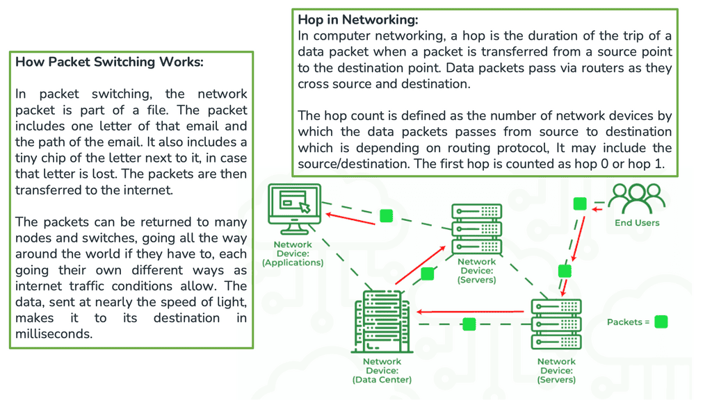
**Datagram networks**
Datagram networks are similar to postal networks. Letters sent between people do not require a connection beforehand. Instead, they can provide their address information by dropping the note off at the local post office. A letter is sent to another post office closer to the destination by the post office. The letter traverses a set of post offices to reach the local post office.
A packet in a datagram network includes the source and destination addresses. Packets are sent to the nearest network device, which passes them on to a device closer to the destination. Network devices make routing decisions, also known as forwarding decisions, when they receive packets. This can be determined using the packet’s destination address and routing table. Each intermediate device decides for each packet.
Example: IPv6 Connectivity
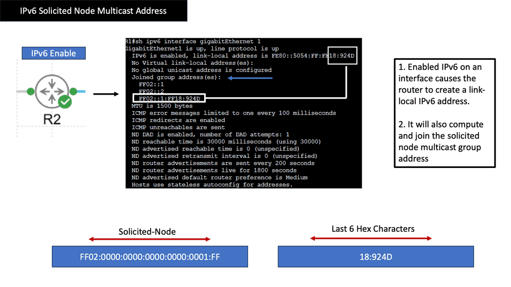
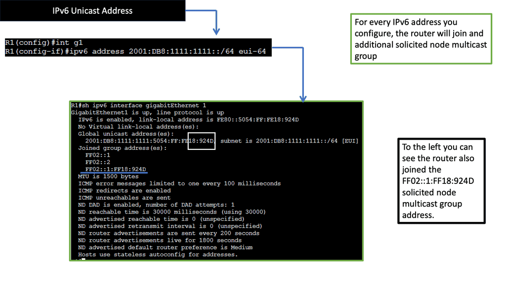
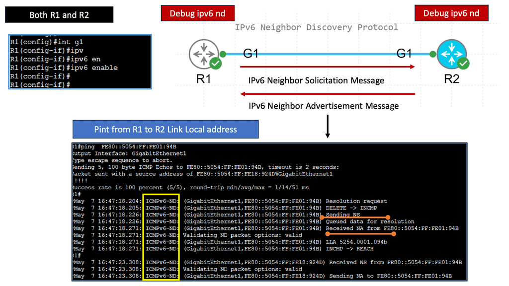
Understanding IPv6 Solicited Node Multicast Address
The IPv6 Solicited Node Multicast Address is a unique feature of IPv6 that facilitates efficient communication between hosts on a local network. It is used for various essential functions, such as neighbor discovery, address resolution, and duplicate address detection. This section will provide an in-depth explanation of how the Solicited Node Multicast Address is constructed and operated.
One of the primary purposes of the IPv6 Solicited Node Multicast Address is to enable efficient neighbor discovery and address resolution. This section will explore how hosts utilize the Solicited Node Multicast Address to discover and communicate with neighboring devices. We will delve into the Neighbor Solicitation and Neighbor Advertisement messages, highlighting their role in maintaining an updated Neighbor cache.
Duplicate Address Detection
Ensuring unique and non-conflicting IP addresses is crucial in any network environment. IPv6 Solicited Node Multicast Address is vital in the Duplicate Address Detection (DAD) process. This section will explain how Solicited Node Multicast Address is used to verify the uniqueness of an IP address during the initialization phase, preventing address conflicts and ensuring seamless network operation.
Using IPv6 Solicited Node Multicast Address brings several benefits to modern networking. This section will discuss the advantages of using Solicited Node Multicast Address, such as reduced network traffic, improved efficiency, and enhanced scalability. We will explore real-world scenarios where a Solicited Node Multicast Address proves highly advantageous.
Understanding IPv6 Neighbor Discovery Protocol
The IPv6 Neighbor Discovery Protocol, or NDP, is a core component of the IPv6 protocol suite. It replaces the Address Resolution Protocol (ARP) used in IPv4 networks. NDP offers a range of functions, including address autoconfiguration, neighbor discovery, and router discovery. These functions are essential for efficient communication and smooth operation of IPv6 networks.
a) Neighbor Discovery: One of the primary functions of NDP is to identify and keep track of neighboring devices on the same network segment. Through neighbor discovery, devices can learn each other’s IPv6 addresses, link-layer addresses, and other vital information necessary for communication.
b) Address Autoconfiguration: NDP simplifies assigning IPv6 addresses to devices. With address autoconfiguration, devices can generate unique addresses using network prefixes and interface identifiers. This eliminates manual IP address assignment and significantly streamlines network setup.
c) Router Discovery: NDP allows devices to discover routers on the network without relying on a predefined configuration. By periodically sending Router Advertisement (RA) messages, routers announce their presence, network prefixes, and other configuration options. This enables devices to dynamically adapt to changes in the network topology and maintain seamless connectivity.
Benefits of IPv6 Neighbor Discovery Protocol
a) Efficient Network Operations: NDP reduces the reliance on manual configuration, making network setup and management more efficient. With autoconfiguration and neighbor discovery, devices can seamlessly join or leave the network without extensive administrative intervention.
b) Enhanced Security: NDP incorporates security features such as Secure Neighbor Discovery (SEND), which protects against attacks such as neighbor spoofing and rogue router advertisements. SEND ensures the integrity and authenticity of NDP messages, bolstering the overall security of IPv6 networks.

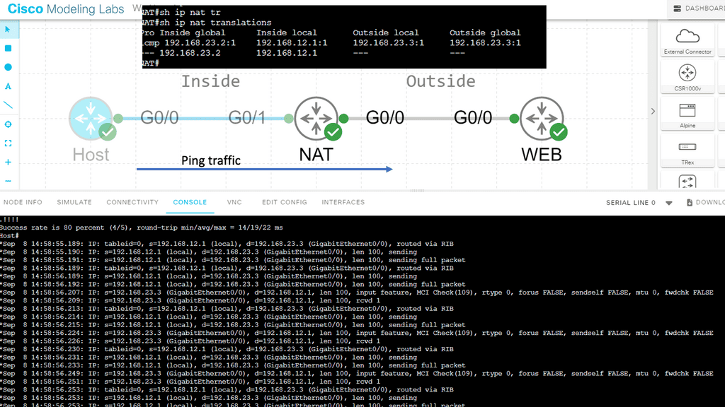
IP Forwarding and NAT
In addition to interconnecting networks, IP forwarding enables network address translation (NAT). NAT allows multiple devices within a private network to share a single public IP address. When a device from the private network sends an IP packet to the internet, the router performing NAT modifies the packet’s source IP address to the public IP address before forwarding it. This allows the device to communicate with the internet using a single public IP address, effectively hiding the internal network structure.
Example Technology: IPv6 NAT
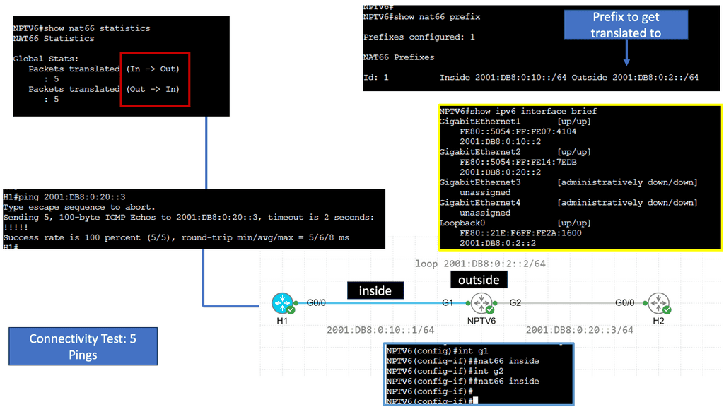
Understanding NPTv6
NPTv6, also known as Network Prefix Translation for IPv6, is a mechanism designed to facilitate the transition from IPv4 to IPv6. It enables communication between IPv6 and legacy IPv4 networks by performing address translation. Unlike conventional IPv6 transition mechanisms, NPTv6 eliminates the need for tunneling or dual-stack deployment, making it an attractive solution for organizations seeking a smooth transition to IPv6.
One of NPTv6’s key advantages is its ability to simplify network management. By enabling seamless communication between IPv6 and IPv4 networks, organizations can adopt IPv6 incrementally without disrupting their existing infrastructure. Additionally, NPTv6 provides address independence, allowing devices within an IPv6 network to communicate with the outside world using a single, globally routable IPv6 prefix.
Implementation Challenges
While NPTv6 offers numerous benefits, it is not without its implementation challenges. One significant challenge is the potential impact on network performance. Since NPTv6 involves address translation, there may be a slight increase in latency and processing overhead. Organizations must carefully evaluate their network infrastructure and consider scalability and performance implications before implementing NPTv6.
As the world becomes increasingly reliant on IPv6, NPTv6 is poised to play a pivotal role in shaping the future of networking. Its ability to bridge the gap between IPv6 and IPv4 networks opens up new possibilities for seamless communication and global connectivity. With the proliferation of IoT devices and the need for efficient and secure networks, NPTv6 offers a scalable solution that accommodates the digital era’s growing demands.
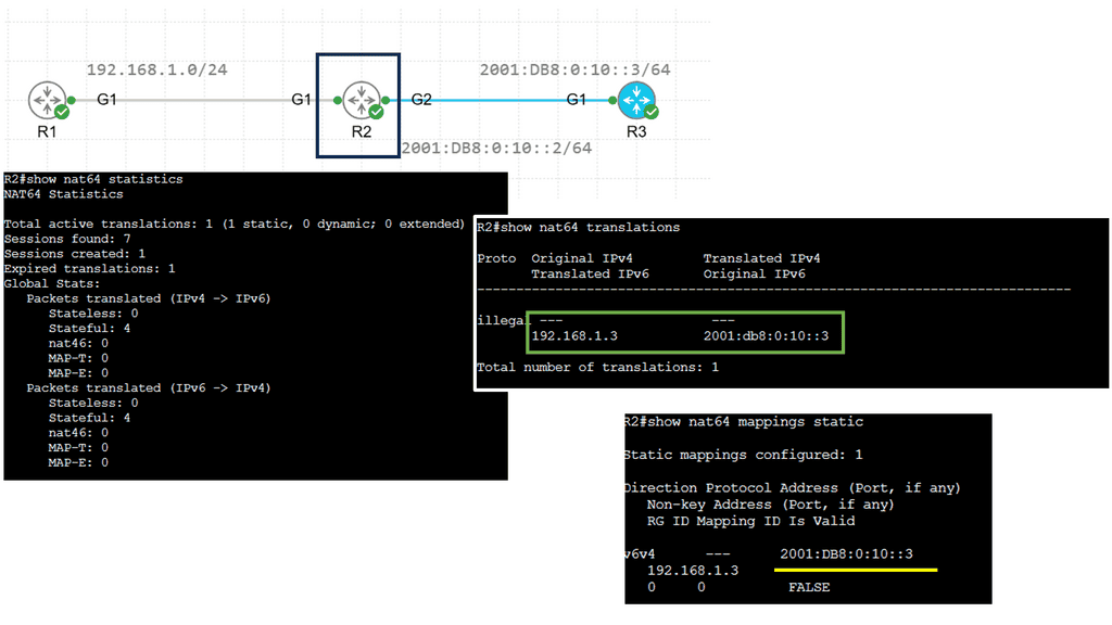
Example: NAT64 Static Configuration
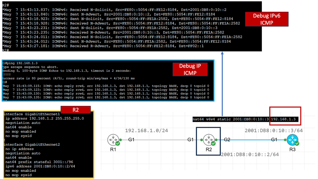
Understanding NAT64
NAT64, which stands for Network Address Translation 64, is a mechanism that facilitates communication between IPv6 and IPv4 networks. It acts as a translator, allowing devices using different IP versions to communicate seamlessly. By mapping IPv6 addresses to IPv4 addresses and vice versa, NAT64 enables cross-network compatibility.
Implementing NAT64 brings a myriad of advantages. Firstly, it enables IPv6-only devices to communicate with IPv4 devices without complex dual-stack configurations. This simplifies network management and reduces the burden of maintaining IPv4 and IPv6 infrastructures. Additionally, NAT64 provides a smooth transition path for organizations migrating from IPv4 to IPv6, allowing them to adopt the new protocol while ensuring connectivity with legacy IPv4 networks.
To implement NAT64, a NAT64 gateway is required. This gateway acts as an intermediary between IPv6 and IPv4 networks, performing address translation as packets traverse. Various open-source and commercial solutions are available for deploying NAT64 gateways, offering flexibility and options based on specific network requirements.
Advanced Topic
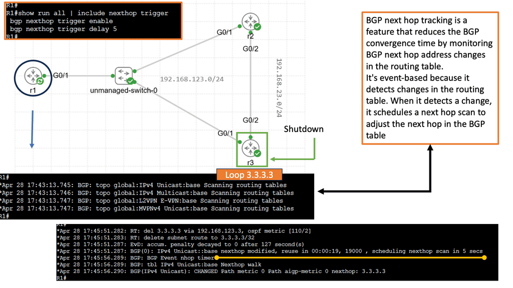
Understanding BGP Next Hop
BGP Next Hop refers to the IP address to which a router forwards packets destined for a specific network. Traditionally, the next hop address remains unchanged in the BGP routing table, irrespective of the underlying network conditions. However, with Next Hop Tracking, the next hop address dynamically adjusts based on real-time monitoring and evaluation of network paths and link availability.
Enhanced Network Resiliency: By continuously monitoring the status of network paths, BGP Next Hop Tracking enables routers to make informed decisions in the face of link failures or congestion. Routers can swiftly adapt and reroute traffic to alternate paths, thus minimizing downtime and improving network resiliency.
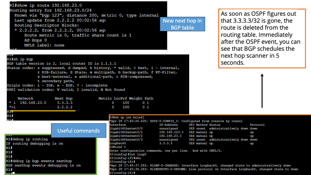
Enabling Next Hop Tracking: Network operators must configure their routers to exchange BGP updates, including the Next Hop Tracking attribute, to allow BGP to Next Hop Tracking. This attribute carries information about the status and availability of alternate paths, allowing routers to make informed decisions when selecting the next hop.
Adjusting Next Hop Metric: Network administrators can also customize the metric used for Next Hop Tracking. Administrators can influence routers’ decision-making process by assigning weights or preferences to specific paths, ensuring traffic is routed as desired.
Next Hop Tracking empowers network administrators to fine-tune traffic engineering policies. Administrators can intelligently distribute traffic across multiple paths by considering link utilization, latency, and available bandwidth, ensuring optimal resource utilization and improved network performance.
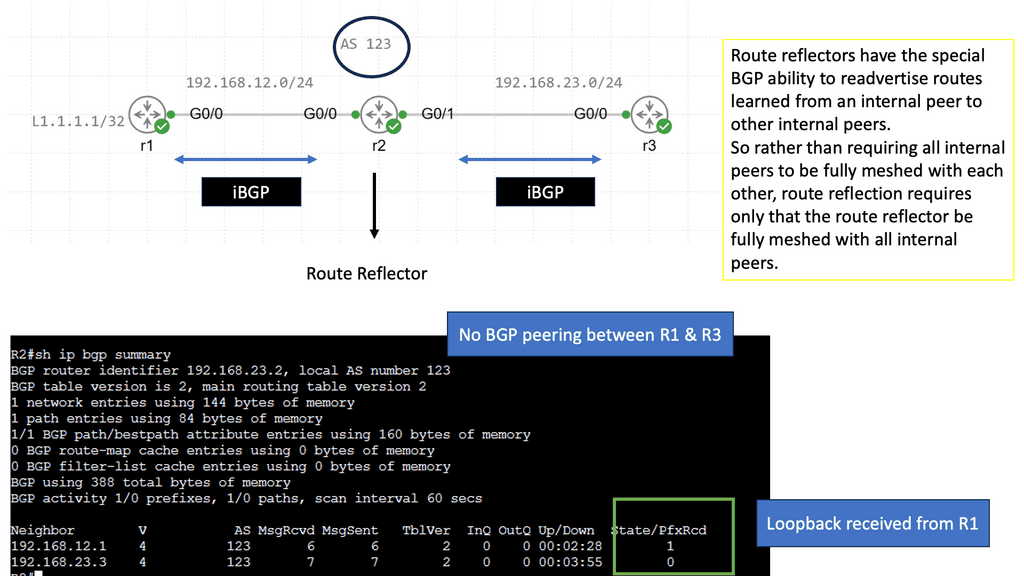
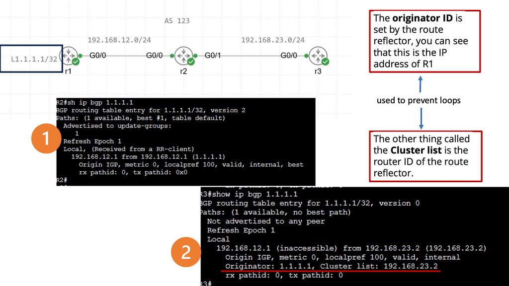
Understanding BGP and Its Challenges
BGP, the internet’s de facto interdomain routing protocol, is designed to exchange routing information between autonomous systems (ASes). However, as networks grow in size and complexity, challenges arise regarding scalability, convergence, and the propagation of routing updates. These challenges necessitate the use of mechanisms like route reflection.
Route reflection is a technique employed in BGP to reduce the number of full-mesh connections required in a network by allowing route reflectors to act as intermediaries between BGP speakers. The route reflector receives BGP updates from its clients and reflects them to other clients, simplifying the topology and reducing the number of required BGP sessions. This enables efficient propagation of routing information within a network.
The implementation of route reflection brings several benefits to network operators. Firstly, it reduces the required BGP sessions, leading to lower resource consumption and improved scalability. Secondly, it enhances convergence time by eliminating the need for full-mesh connectivity. Additionally, route reflection aids in reducing the complexity of BGP configurations, making network management more manageable and less error-prone.
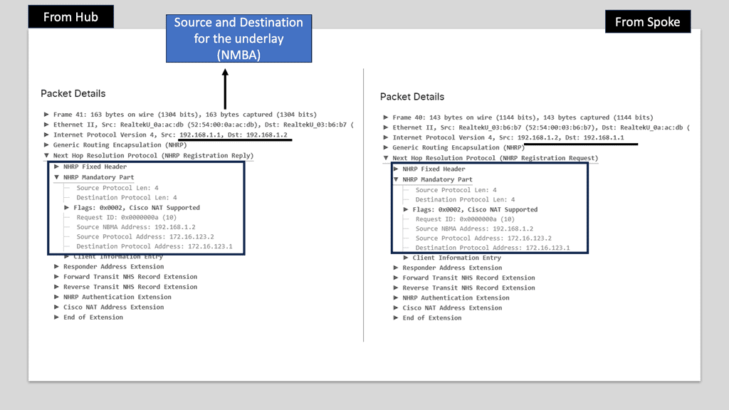
Understanding Next Hop Redundancy Protocol
NHRP, a routing protocol designed for multipoint networks, is crucial in providing redundancy and enhancing network reliability. Eliminating single points of failure enables seamless communication even in the face of link failures or network congestion. Let’s explore how NHRP achieves this.
The underlay functionality of NHRP focuses on establishing and maintaining direct communication paths between network devices. It utilizes Address Resolution Protocol (ARP) to map logical to physical addresses, ensuring efficient routing within the underlay network. By dynamically updating and caching information about network devices, NHRP minimizes latency and data transmission.
In addition to its underlay capabilities, NHRP also provides overlay functionality. This enables communication between devices across different network domains, utilizing overlay tunnels. By encapsulating packets within these tunnels and dynamically discovering the most efficient paths, NHRP ensures seamless connectivity and load balancing across the overlay network.


Related: Before you proceed, you may find the following post helpful for pre-information:
IP routing is the process by which routers forward IP packets. Routers have to take different steps when forwarding IP packets from one interface to another, which has nothing to do with the “learning” of network routes via static or dynamic routing protocols.
IP Forwarding
Before you get into the details, let me cover the basics. A router receives a packet on one of its interfaces and then forwards the packet out of another based on the contents found in the IP header. For example, if the packet were part of a video stream ( Multicast / multi-destination), it would be forwarded to multiple interfaces. If the packet were part of a typical banking transaction ( Unicast ), it would be forwarded to one of its interfaces.
As each routing device forwards the packet hop-by-hop, the packet’s IP header remains relatively unchanged, containing complete instructions for forwarding the packet. However, the data link headers ( the layer directly below ) may change radically at each hop to match the changing media types.
For example, the router receives a packet on one of its attached Ethernet Segments. The routers will first look at the packet’s data-link header, which is Ethernet. If the Ethertype is set to (0x800 ), indicating an IP packet ( A unicast MPLS packet has an Ethertype value of 0x8847 ), the Ethernet header is stripped from the packet, and the IP header is examined.
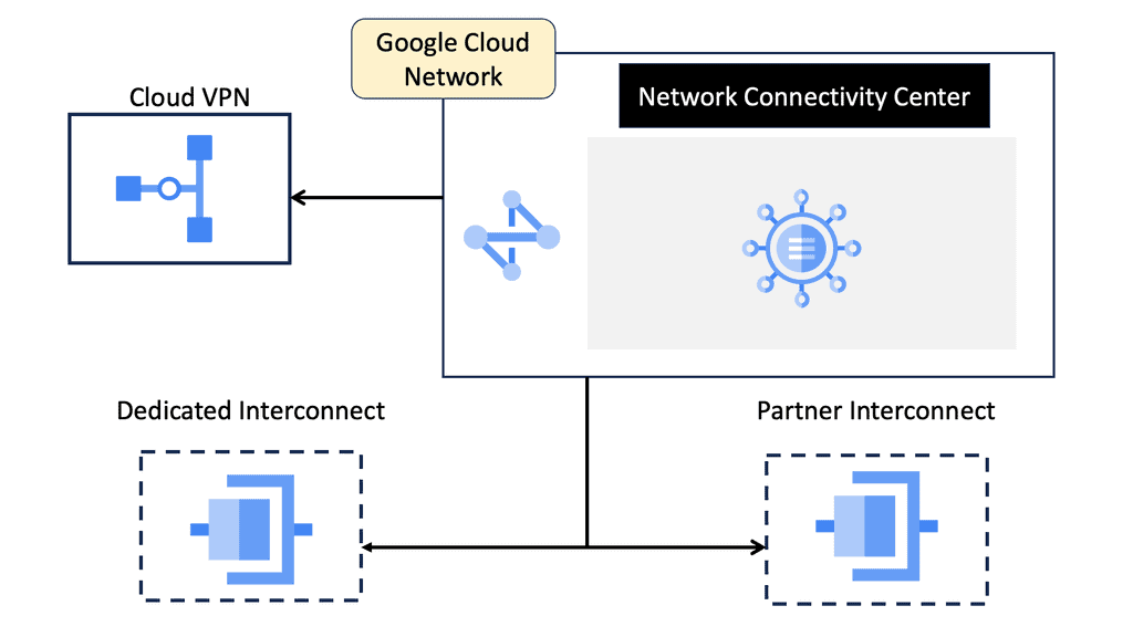
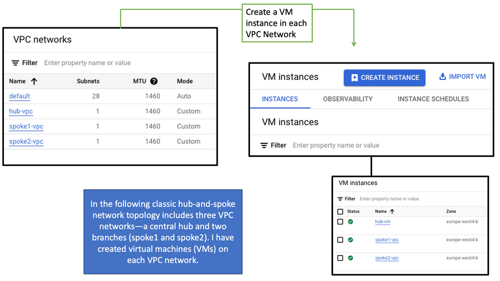
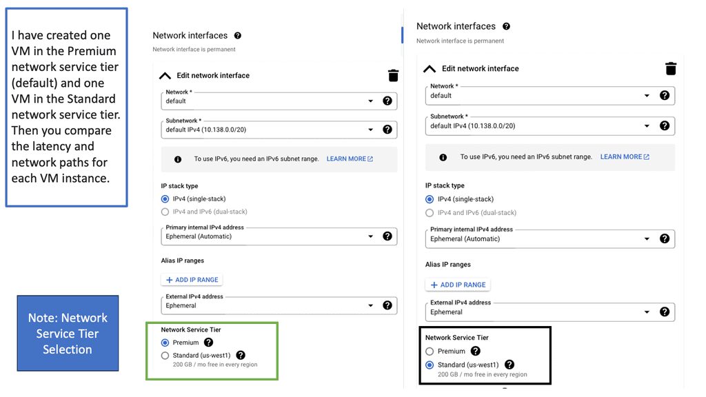
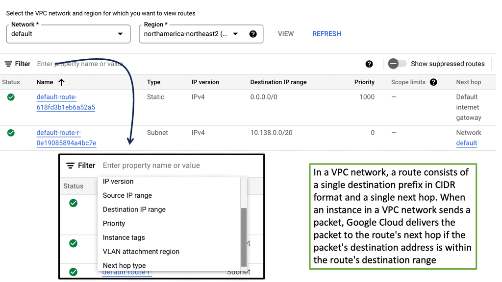
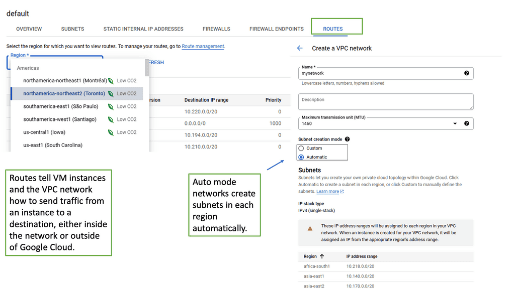
Understanding VPC Networking
Before we dive into Google Cloud’s VPC networking, let’s gain a basic understanding of what VPC networking entails. VPC, which stands for Virtual Private Cloud, allows you to create your own isolated virtual network in the cloud. It provides control over IP addressing, routing, and network access for your resources deployed in the cloud.
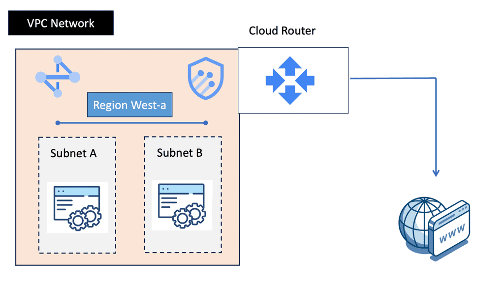
Google Cloud’s VPC networking offers a range of powerful features that enhance network security, performance, and scalability. Some of these features include:
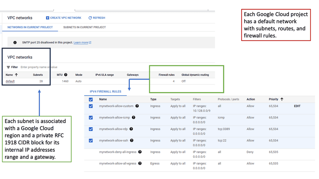
1. Subnets and IP Address Management: With Google Cloud VPC, you can create multiple subnets within a VPC, each with its own IP address range. This allows you to segment your network and control traffic flow effectively.
2. Firewall Rules: Google Cloud provides a robust firewall solution that allows you to define granular access control policies for your VPC. You can create firewall rules based on source IP, destination IP, ports, and protocols, ensuring secure network communication.
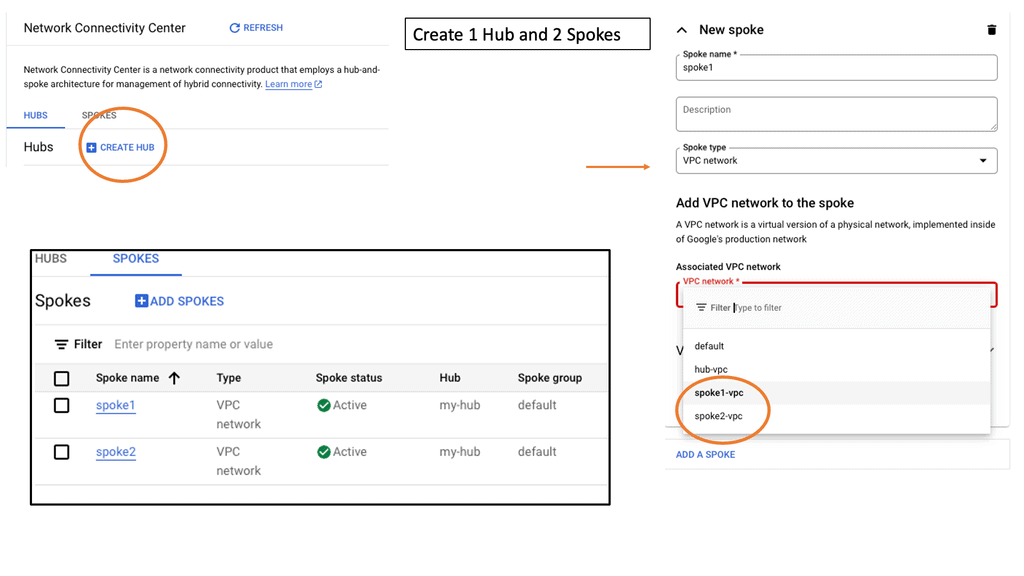
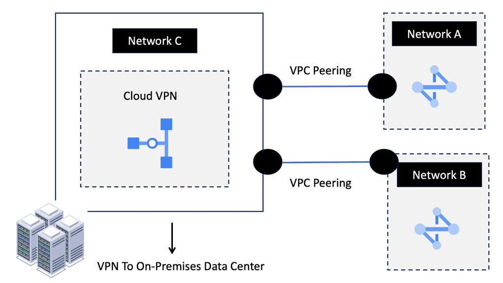
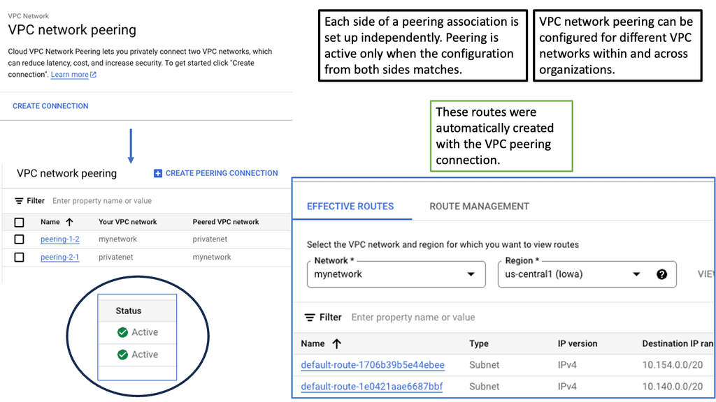
3. VPC Peering: VPC peering enables you to establish private connectivity between VPC networks, both within Google Cloud and with external networks. This allows for seamless communication between resources across different VPCs.
4. Cloud VPN and Cloud Interconnect: Google Cloud offers VPN and dedicated interconnect options to establish secure and high-performance connections between your on-premises infrastructure and Google Cloud VPC networks.
The “learning” of network routes
IP packet forwarding has nothing to do with the “learning” of network routes carried out through static or dynamic routing protocols. Instead, IP forwarding has everything to do with routers’ steps when they forward an IP packet from one interface to another.
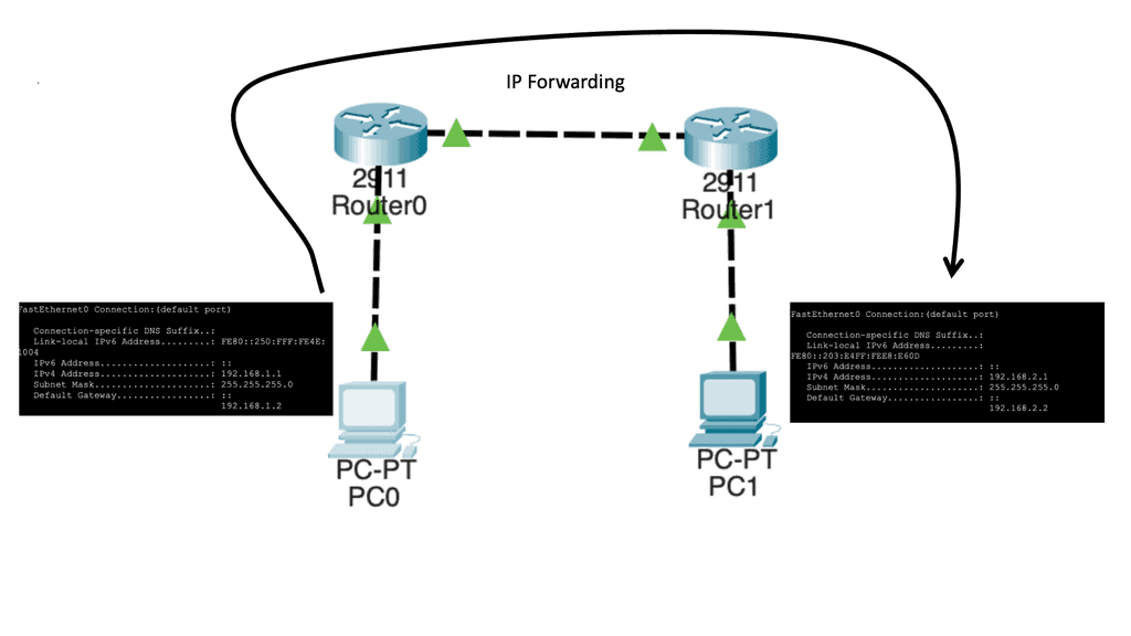
Let us say we have two host computers and two routers. Host1, on the left, will send an IP packet to Host2, which is on the right. This IP packet has to be routed by R0 and R1. Host 1 is on 192.168.1.0/24, and Host 2 is on 192.168.2.0/24
Let’s start with Host1, which creates an IP packet with its IP address (192.168.1.1) as the source and Host 2 (192.168.2.1) as the destination. So the first question that Host1 will need to determine:
- Question: Is the destination I am trying to reach either local or remote?
To get the answers to this question, look at its IP address, subnet mask, and destination IP address.
1st Lab Guide: IP Forwarding
Our network has Host1, which is in network 192.168.1.0/24. As a result, all IP addresses in the 192.168.1.1 – 254 range are local. Unfortunately, our destination (192.168.2.1, which is the remote Host) is outside the local subnet, so we must use the default gateway. In our case, the default gateway is the connected router.
Therefore, Host 1 will build an Ethernet frame and enter its source MAC address. Host 1 then has to ask itself another question. What is the destination MAC address of the default gateway, the connected router?
Analysis:
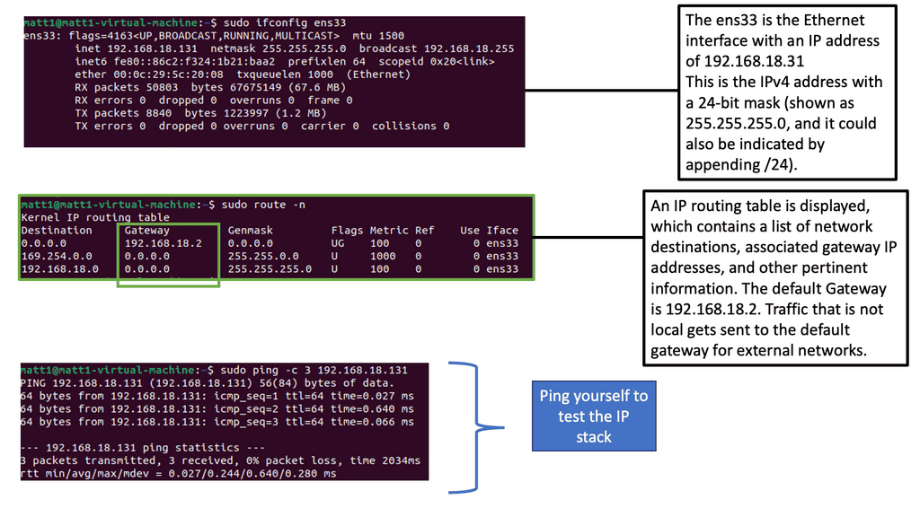
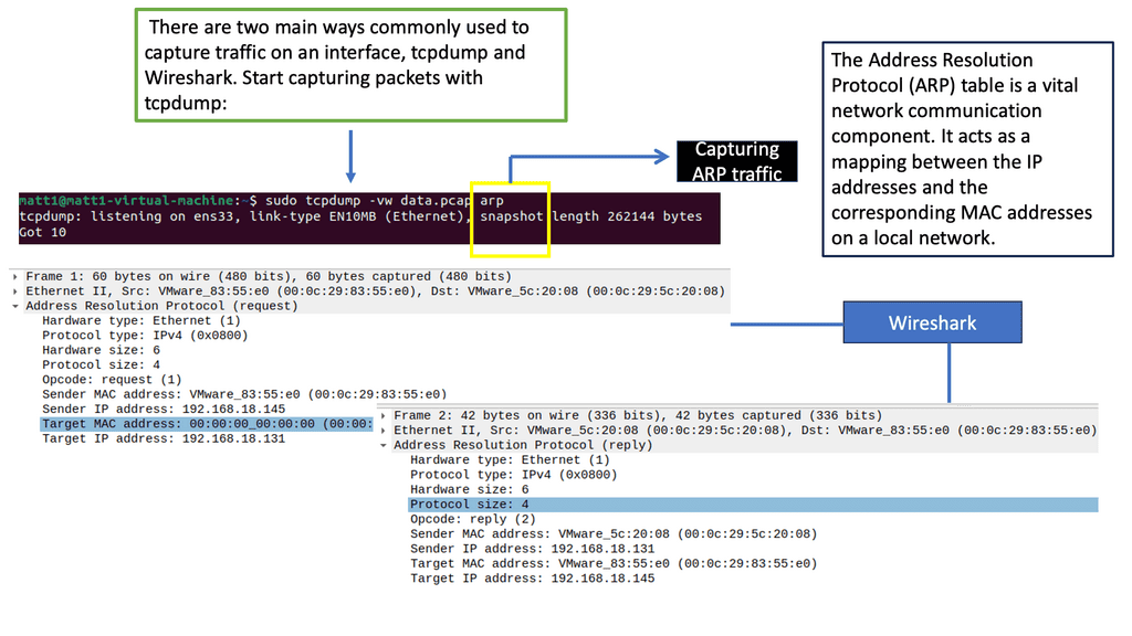
To determine this, the Host checks its ARP table to find the answer. In our case, Host1 has an ARP entry for 192.168.1.2, the default gateway. It has an ARP entry, as I did a quick testing ping before I took the screenshot. It is a dynamic entry, not a static one, as I did not manually enter this MAC address. If the Host did not have an APR entry, it would have sent an ARP request.
Note:
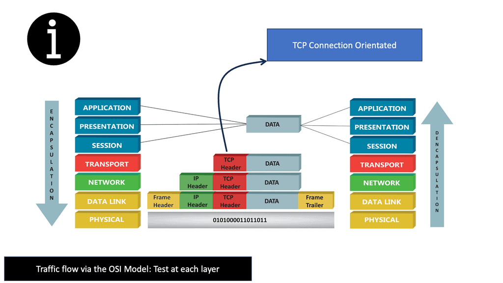
Ping uses the ICMP protocol, and IP uses the network layer (layer 3). Our IP packet will have a source IP address of 192.168.1.1 and a destination IP address of 192.168.1.2. The next step is to put our IP packet in an Ethernet frame, where we set our source MAC address PC0 and destination MAC address PC1.
Now, wait a second. How does PC0 know the MAC address of PC1? We know the IP address because we typed it, but H1 cannot identify the MAC address of H2. Another protocol that will solve this problem is ARP (Address Resolution Protocol).
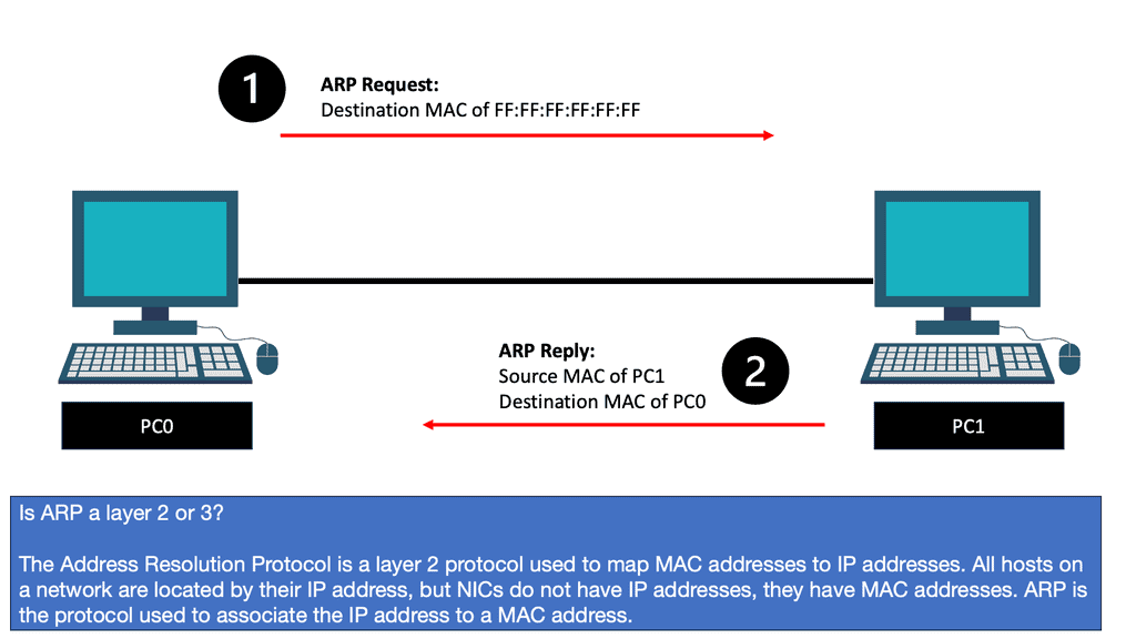
So, with ARP, I have the IP address, and I want to find out the MAC address as we move down the OSI model’s layers so bits can be forwarded on the wire. At this stage, the Ethernet frame carries an IP packet. Then, the frame will be on its way to the directly connected router.
In the network topology at the start of the lab guide, the Ethernet frame makes it to R0. So, as this is a Layer 3 router and not a Host or Layer 2 switch, it has more work. So the first thing it does is check if the FCS (Frame Check Sequence) of the Ethernet frame is correct or not:
If the FCS is incorrect, the frame is dropped right away. Unfortunately, Ethernet has no error recovery; this is done by protocols on upper layers, like TCP on the transport layer.
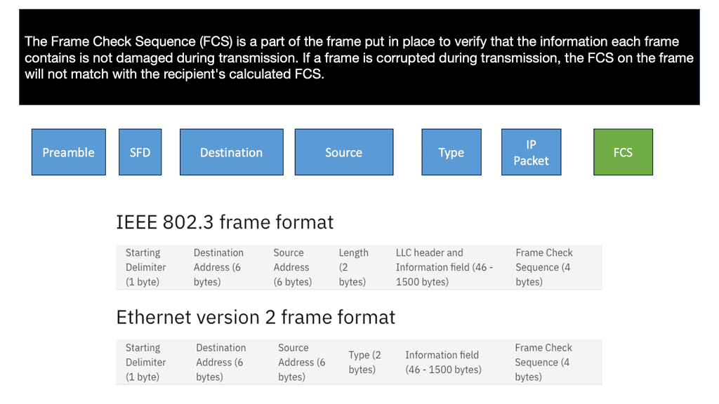
If the FCS is correct, we will process the frame if:
- The destination MAC address is the address of the router interface.
- The destination MAC address is the subnet’s broadcast address to which the router interface is connected.
- The destination MAC address is a multicast address that the router listens to.
Note:
In our case, the destination MAC address matches the MAC address of R0’s GigabitEthernet 0/0 interface. Therefore, the router will process it. But, first, we de-encapsulate ( which means we will extract) the IP packet out of the Ethernet frame, which is then discarded:
The router, R0, will now look at the IP packet, and the first thing it does is check if the header checksum is OK. Remember that there is also no error recovery on the Layer 3 network layer; we rely on the upper layers. Then R0 checks its routing table to see if there is a match:
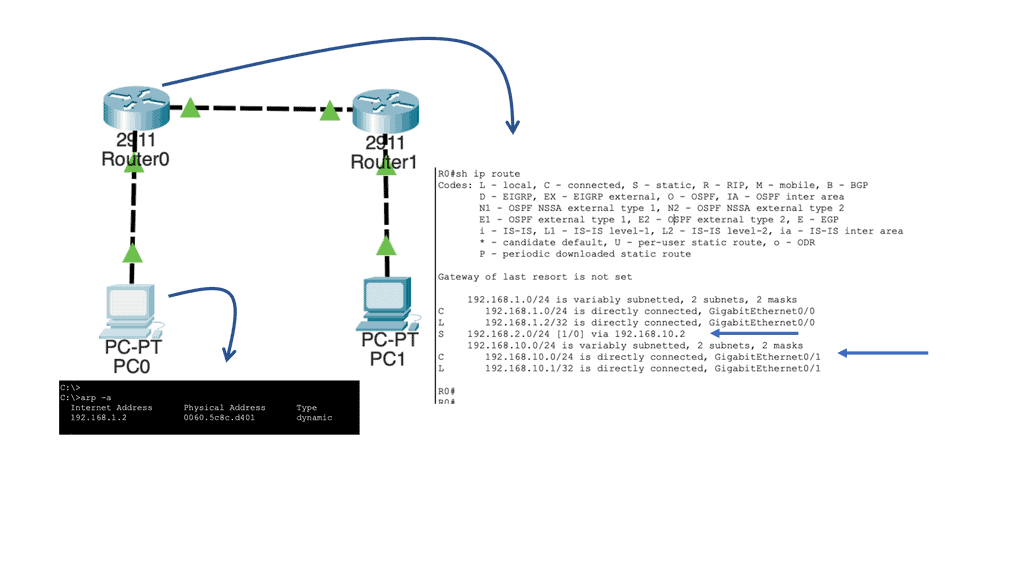
Above, you can see that R0 knows how to reach the 192.168.2.0/24 network. This is because the destination address has a next-hop IP address, 192.168.10.2, which is the connecting Router – R1.
It will now do a second routing table lookup to see if it can reach 192.168.10.2. This is called recursive routing. The Recursive Route Lookup follows the same logic of dividing a task into subtasks of the same type. The device repeatedly performs its routing table lookup until it finds the ongoing interface to reach a particular network.
As you can see above, there is an entry for 192.168.10.0/24 with GigabitEthernet 0/1 as the interface. Once this is done, R0 checks its local ARP table to determine if there is an entry for 192.168.10.2. Similar to the sending Host, if there were no ARP entries, R0 would have to send an ARP request to find the MAC address of 192.168.10.2.
The next stage is that R0 builds a new Ethernet frame with its MAC address of the GigabitEthernet 0/1 interface and R1 as the destination. The IP packet is then encapsulated in this new Ethernet frame.
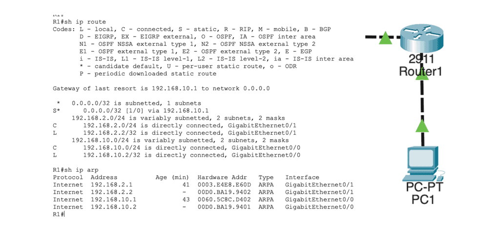
In the routing table, we find this:
Network 192.168.2.0/24 directly connects to R1 on its GigabitEthernet 0/1 interface. R1 will now reduce the IP packet’s TTL from 254 to 253, recalculate the IP header checksum, and check its ARP table to see if it knows how to reach 192.168.2.1. There is an ARP entry there. The new Ethernet frame is created, and the IP packet is encapsulated. Host2 then looks for the protocol field to determine what transport layer protocol we are dealing with; what happens next depends on the protocol used.
Note: The TTL represents a field in IP packets that helps prevent infinite loops and ensures the proper functioning of routing protocols. As a packet traverses through routers, the TTL value gets decremented, and if it reaches zero, the packet is discarded. This mechanism prevents packets from endlessly circulating in a network, facilitating efficient and reliable data transmission.
Knowledge Check: ICMP ( Internet Control Message Protocol )
What is ICMP?
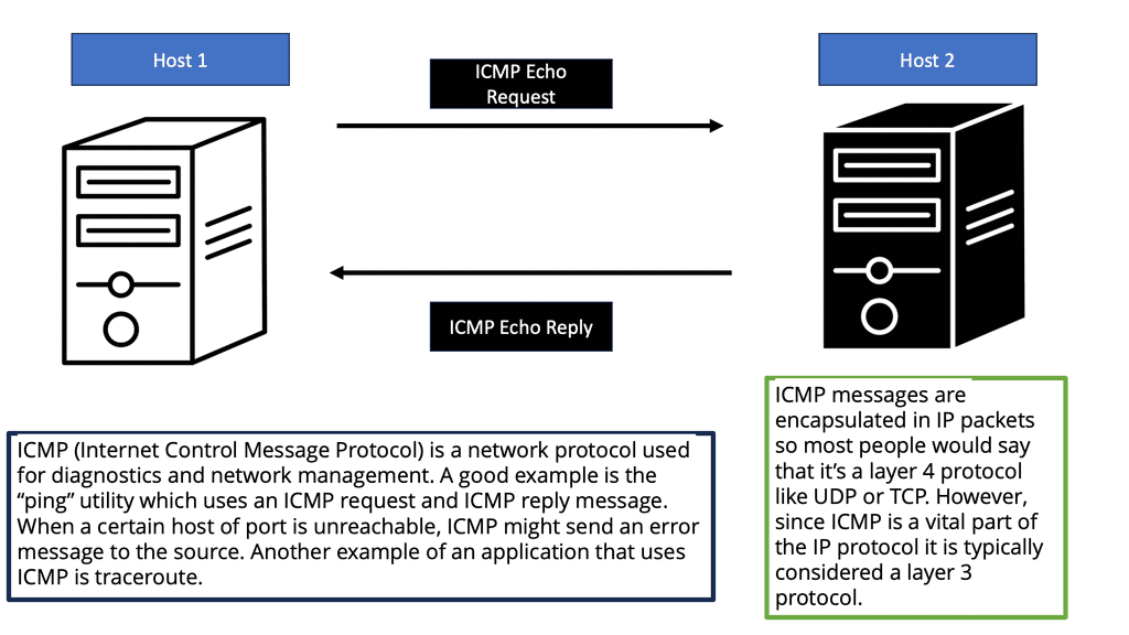
ICMP is a protocol that operates at the network layer of the Internet Protocol Suite. Its primary purpose is to report and diagnose errors that occur during the transmission of IP packets. ICMP messages are typically generated by network devices, such as routers or hosts, to communicate vital information to other devices in the network.
ICMP Functions and Types
ICMP serves several functions, but its most common use is error reporting. When a network device encounters an issue while transmitting an IP packet, it can use ICMP to send an error message back to the source device. This enables the source device to take appropriate action, such as retransmitting the packet or choosing an alternative route.
ICMP messages come in different types, each serving a specific purpose. Some commonly encountered ICMP message types include Destination Unreachable, Time Exceeded, Echo Request, and Echo Reply. Each type has its unique code and is crucial in maintaining network connectivity.
ICMP and Network Troubleshooting
ICMP is an invaluable tool for network troubleshooting. Providing error reporting and diagnostic capabilities helps network administrators identify and resolve network issues more efficiently. ICMP’s ping utility, for example, allows administrators to test a remote host’s reachability and round-trip time. Traceroute, another ICMP-based tool, helps identify the path packets take from the source to the destination.
ICMP and Network Security
While ICMP serves critical networking functions, it is not without its security implications. Certain ICMP message types, such as ICMP Echo Request (ping), can be abused by malicious actors for reconnaissance or denial-of-service attacks. Network administrators often implement security measures, such as ICMP rate limiting or firewall rules, to mitigate potential risks associated with ICMP-based attacks.
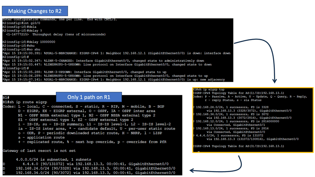
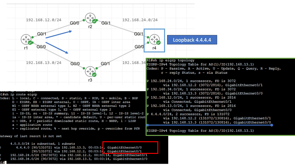
Guide: EIGRP and the Variance Command
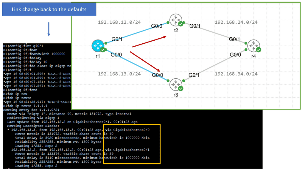
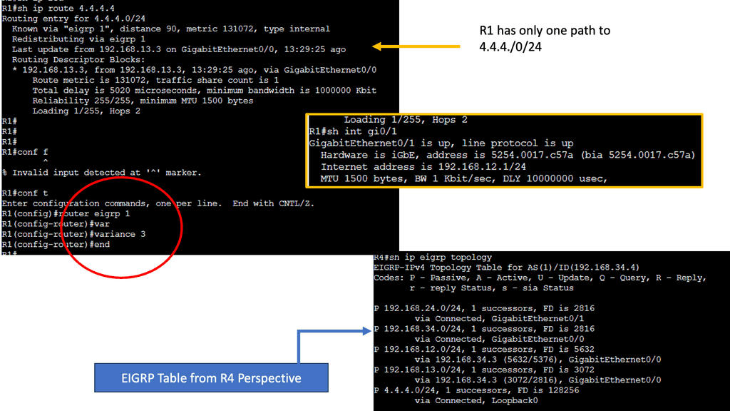
EIGRP operates at the network layer and uses a distance-vector routing algorithm. It is designed to exchange routing information efficiently, calculate the best paths, and adapt to network changes. Cisco EIGRP offers a range of advanced features that can enhance network performance and scalability. We will explore features such as route redistribution, load balancing, and stub routing. In this guide, I will look at the EIGRP variance feature. Below, I have 4 routers. I have changed the bandwidth and delay. Once changed, the routing table only shows one path to the 4.4.4.4 loopback connected to R4.

Understanding EIGRP Variance
EIGRP, or Enhanced Interior Gateway Routing Protocol, is a dynamic routing protocol widely used in enterprise networks. By default, EIGRP only allows load balancing across equal-cost paths. However, in scenarios where multiple paths have varying costs, the EIGRP variance command comes to the rescue. It enables load balancing across unequal-cost paths, distributing traffic more efficiently and effectively.
Configuring EIGRP Variance
Configuring the EIGRP variance command is relatively straightforward. First, you need to access the router’s command-line interface. Once there, you can enter the global configuration mode and specify the variance value. The variance value represents the multiplier determining the feasibility condition for unequal-cost load balancing. For instance, a variance of 2 means that a path with a metric up to two times the best path metric is considered feasible.
Impact on Network Performance
The EIGRP variance command significantly impacts network performance. It effectively utilizes network resources and improves overall throughput by allowing load balancing across unequal-cost paths. Additionally, it enhances network resilience by providing alternative paths in case of link failures. However, it’s important to note that deploying the EIGRP variance command requires careful consideration of network topology and link costs to ensure optimal results.
**Inter-network packet transfer**
IP forwarding is used for inter-network packet transfer and not for inter-interface transfers. Therefore, if two interfaces are on the same network, we don’t need to enable IP forwarding.
Let us look at an example of IP forwarding. Consider a server with two physical ethernet ports, such as your internal network and the outside world, as a DSL modem provides. The system can communicate on either network if you connect and configure those two interfaces. However, packets from one network cannot travel to another if forwarding is not enabled.
IP forwarding determines which path a packet or datagram can be sent. The process uses routing information to make decisions and is designed to send a packet over multiple networks. Generally, networks are separated from each other by routers.

IP Forwarding Example: Verifying the IP Header
The router then verifies the IP header’s contents by checking several fields to validate it. In addition, the router should check that the entire packet has been received by checking the IP length against the size of the received Ethernet packet. If these basic checks fail, the packet is deemed malformed and discarded.
Next, the router verifies the TTL field in the IP header and determines that it is greater than 1. The Time-To-Live field ( TTL ) specifies how long the packet should live, and its value is counted in terms of the number of routers the packet ( technically a datagram ) has traversed ( hop count ).
IP Forwarding Example: The TTL values
The source host selects the initial TTL value and is recommended to use 64. In specific scenarios, other values are set to limit the time, in hops, that the packet should live. The TTL aims to ensure the packet does not circulate forever when there are routing loops. Each router in the path decrements the TTL field by 1 when it forwards the packet out of its interface (s). When the TTL field is decremented to 0, the packet is discarded, and a message known as an ICMP ( Internet Control Message Protocol ) TTL Exceeded is sent back to the host.
IP Forwarding Example: Checking the Destination
For IP forwarding, the router then looks at the destination IP address, which can be either a destination host ( Unicast ), a group of destination hosts ( multicast ), or all hosts on the segment ( broadcast ). As mentioned previously, the router has a routing table that tells it how to forward a packet, and the destination IP address is a crucial component for the routing table lookup.
Forwarding is done on a destination base; if I want to get to destination X, I must go to Y ( the source routing concept is not in this article’s scope). The contents of the router routing table are parsed, and the best-matching routing table entry is returned, indicating whether to forward the packet and, if so, the interface to forward the packet out of and the IP address of the following IP router ( if any ) in the packet’s path.
**The CEF process**
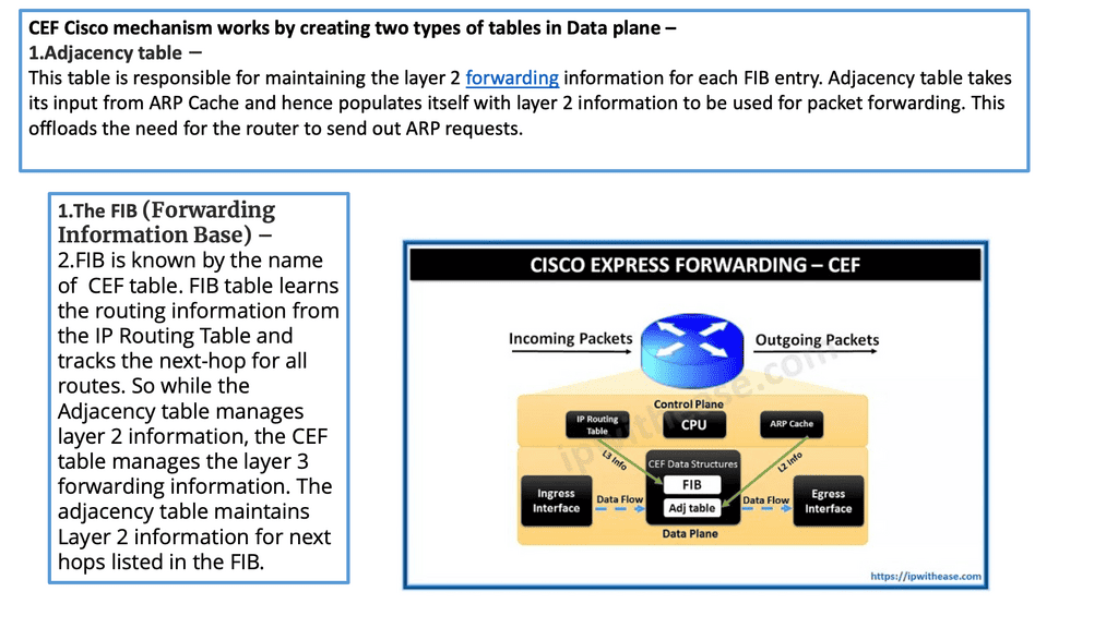
CEFs (Cisco Express Forwarding) are packet-switching technology in Cisco routers. It is designed to enhance network forwarding performance by reducing the overhead associated with Layer 3 forwarding. CEF utilizes a Forwarding Information Base (FIB) and an adjacency table to forward packets quickly to their destinations.
**The FIB Table**
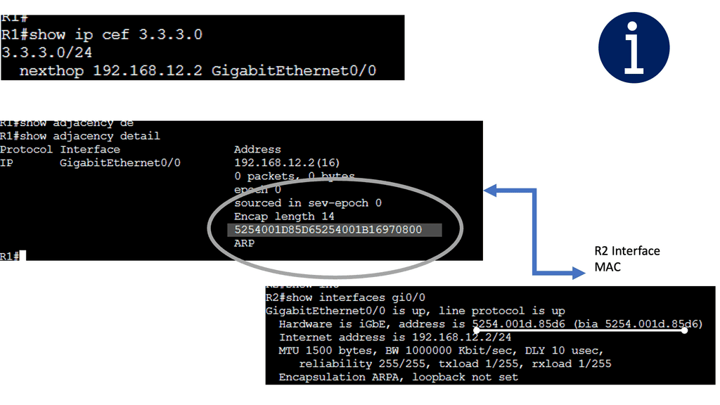
The FIB maintains a list of all known IP prefixes and their associated next-hop addresses. The adjacency table holds information about the Layer 2 addresses of directly connected neighbors. When a packet arrives at a router, the CEF algorithm consults the FIB to determine the appropriate next-hop address. Then, it uses the adjacency table to forward the packet to the correct interface.
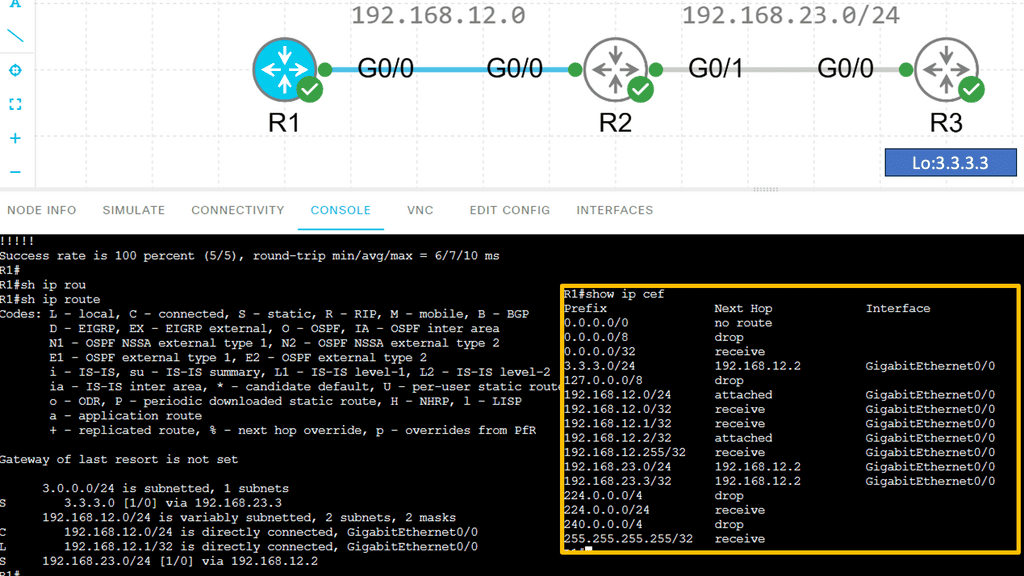
On a Cisco device, the actual moving of the packet from the inbound interface to the outbound interface is carried out by a process known as CEF ( Cisco Express Forwarding ). CEF is a mirror image of the routing table, and any changes in the routing table are reflected in the CEF table. It has a structure different from the routing table, allowing fast lookups.
If you want to parse the routing table, you have to start at the top and work your way down; this can be time-consuming and resource-intensive, especially if your match is the last entry in the routing table. CEF structures let you search on the bit boundary and optimize the routing process with the adjacency table.
Guide: CEF Operations
In this lab guide, I will address CEF operations. There are different switching methods to forward IP packets. Here are the different switching options: Remember that the default is CEF.
- Process switching:
- The CPU examines all packets, and all forwarding decisions are made in software…very slow!
- Fast switching (also known as route caching):
- The CPU examines the first packet in a flow; the forwarding decision is cached in hardware for the next packets in the same flow. This is a faster method.
- (CEF) Cisco Express Forwarding (also known as topology-based switching):
- Forwarding table created in hardware beforehand. All packets will be switched using hardware. This is the fastest method, but it has some limitations. Multilayer switches and routers use CEF.
For example, a multilayer switch will use the information from tables built by the (control plane) to build hardware tables. It will use the routing table to construct the FIB (Forwarding Information Base) and the ARP table to create the adjacency table. This is the fastest switching method because we now have all the information required for layer two and three to forward IP packets in hardware.
Below are three routers and I, using static routing for complete reachability. On R1, let’s look at the routing and CEF tables. Let’s take a detailed look at the entry for network 3.3.3.0 /24:
 Note:
Note:
How Cisco Express Forwarding Works
CEF builds and maintains two fundamental data structures: the FIB and Adjacency Table. The FIB contains information about the best path to forward packets, while the Adjacency Table stores Layer 2 next-hop addresses. These data structures enable CEF to make forwarding decisions quickly and efficiently, resulting in faster packet processing.
Advanced Features and Customization Options
Cisco Express Forwarding offers various advanced features and customization options to meet specific networking requirements. These include features like NetFlow, which provides detailed traffic analysis, and load-balancing algorithms allowing intelligent traffic distribution. Administrators can tailor CEF to optimize network performance and adapt to changing traffic patterns.
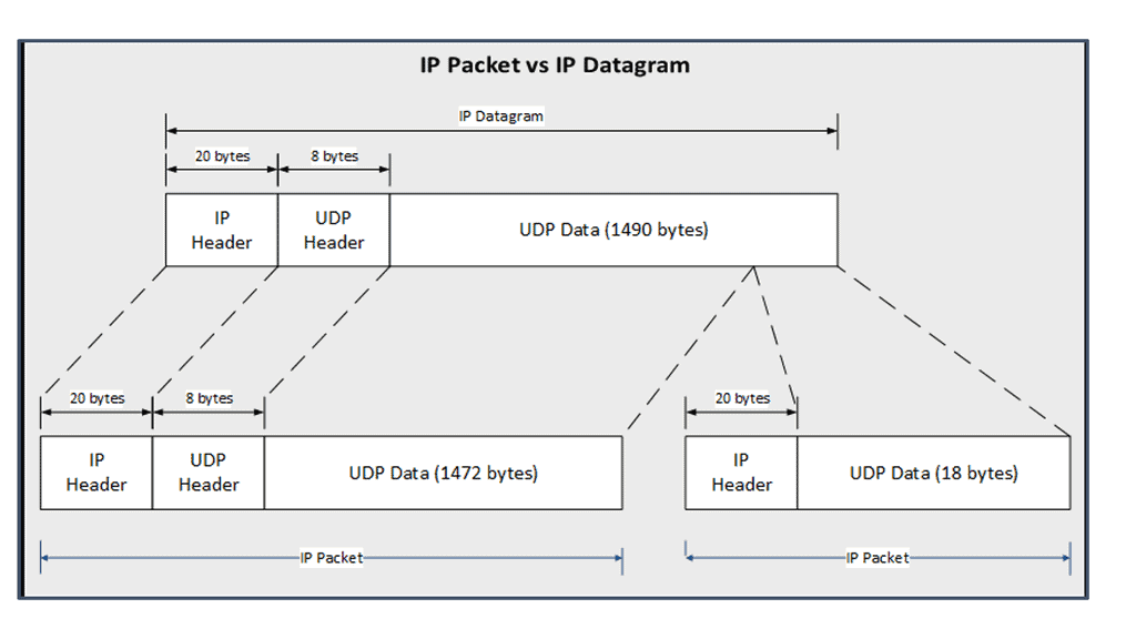
Understanding the MTU
Suppose a router receives a unicast packet too large to be sent out in one piece, as its length exceeds the outgoing interface’s Maximum Transmission Unit ( MTU ). In that case, the router attempts to split the packet into several smaller pieces called fragments. The difference between IPv4 and IPv6 fragmentation is considerable. Slicing packets into smaller packets adversely affects performance and should be avoided.
One way to avoid fragmentation is to have the exact MTU on all links and have the hosts send a packet with an MTU within this range. However, this may not be possible due to the variety of mediums and administrative domains a packet may take from source to destination. Path MTU discovery ( PMTUD ) is the mechanism used to determine the maximum size of the MTU in the path between two end nodes ( source and destination ).
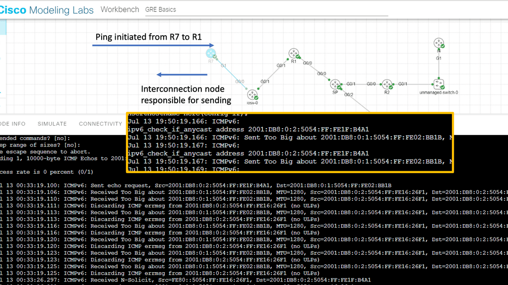
PMTUD
PMTUD dynamically determines the lowest MTU of each link between the end nodes. A host sends an initial packet ( datagram ) with the size of an MTU for that interface, with the DF ( don’t fragment ) bit set.
Any router in the path with a lower MTU discards the packet and returns an ICMP ( Type 4—fragmentation needed and DF set) to the source. This message is also known as a “packet too big” message. The sender estimates a new size for the packet, and the process continues until the PMTU is found.
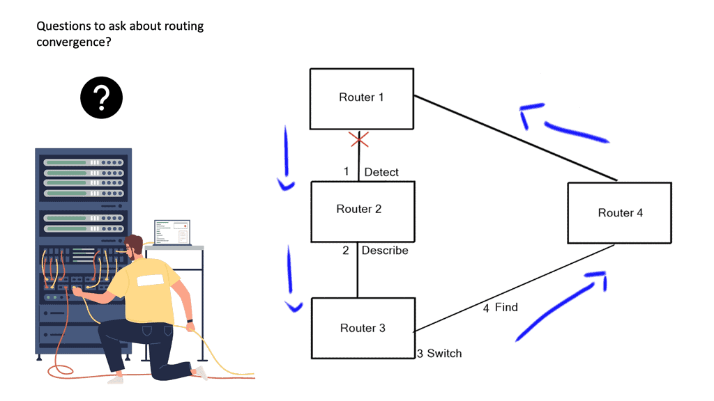
IP Forwarding Example: Modifying the IP Forwarding
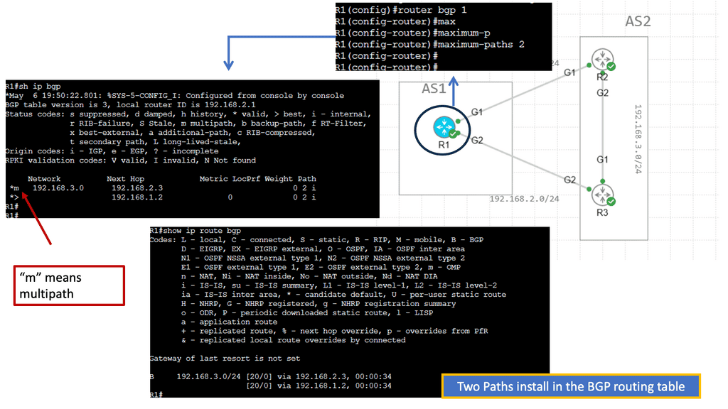
The basics of IP forwarding can be modified in several ways, resulting in data packets taking different paths through the network, some of which are triggered by routing convergence. In previous examples, we discussed routers consulting their routing tables to determine the next hop and single exit interface to send a packet to its destination – “destination-based forwarding. ” However, a router may have multiple paths ( exit interface ) to reach a destination.
These paths can then spread traffic to a destination prefix across alternative links, called multipath routing or load balancing, resulting in more bandwidth available for traffic to that destination.
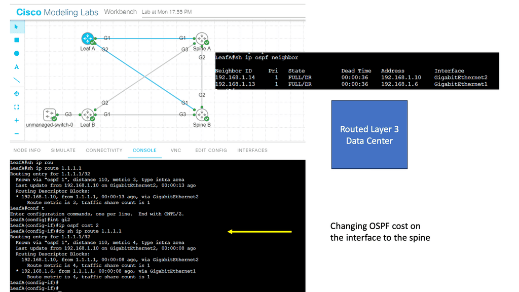
In a layer three environment, links with the exact cost are considered for equal-cost multipathing, and traffic can be load-balanced across those links. You can, however, use unequal-cost links ( links with different costs ) for multipathing, but this needs to be supported in the forwarding routing protocol, e.g., EIGRP.
However, the method used equal or unequal cost multipathing when multiple paths to a destination prefix were used; the router routing table lookup would return numerous next hops. We have the underlay and overlay concept for additional abstracts using the virtual overlay network. They are commonly seen in the Layer-3 data center.
IP Forwarding Example: TCP performance
Generally, routers want to guarantee that packets belonging to a given TCP connection always travel the same path. If done in software, reordering the TCP packets would reduce TCP performance and increase CPU cycles. For this reason, routers use a hash function of some TCP connection identifiers ( source and destination IP address ) to choose among the multiple next hops. A TCP connection is identified by a 5-tuple, which refers to a set of five values that comprise a TCP/IP connection.
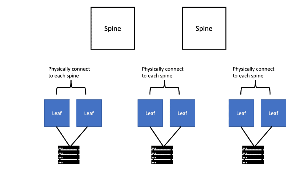
It includes a source IP address/port range, destination IP address/port number, and the protocol in use. A router can load on any of these. In addition, recent availing technologies let L2 load balance ( ECMP ), such as THRILL and Cisco FabricPath, allow you to build massive data center topologies with Layer 2 multipathing. These data centers often operate under a spine-leaf architecture.
IP options
An application can also modify the handling of its packets by extending the IP headers with one or more IP options. IP options are generally used to aid in statistic collection (route record and timestamp) and not to influence path determination as they offer a performance hit. The Internet routers are already optimized for packet forwarding without additional options.
Security devices or filters implemented on routers generally block strict-source and loose-source routes that can be used to control the path packets take. The router then prepends the appropriate data-link header for its outgoing interface. The ARP process then resolves the next-hop IP to the data-link address ( MAC address ), and the router sends the packet to the next hop, where the process is repeated.
A keynote: Ethernet frames have an L2 identifier known as a MAC address, which has 6 bytes for the destination address and 6 bytes for the source address.
The ARP Process
The ARP process is straightforward, translating the IP address ( L3 ) into the associated MAC addresses ( L2 ). Consider the communication between two hosts on an Ethernet segment: Host 1 has an IP address of 10.10.10.1, and Host 2 has an IP address of 10.10.10.2.
For these hosts to communicate, they must build frames at L2 with source and destination hardware MAC addresses. Host 1 opens a web browser and tries to connect to a service on host 2, which has a destination of 10.10.10.2. Host 1 uses ARP to map the IP address to the MAC address of the destination host.
|
The ARP Table
The ARP tables optimize communications between directly connected devices. Upon receiving an ARP response, devices keep the IP-to-MAC address mapping for some time, usually up to 4 hours. This means a router does not need to send an ARP request for any IP address previously learned. ARP tables may also be updated by what is known as a gratuitous ARP. A gratuitous ARP is an ARP request that a host sends to itself to update its neighbors’ ARP tables.
An example is when a VM is moved from one ESX host to another. For the other devices to know it has moved, it sends a gratuitous ARP. This process updates the router’s ARP table. Due to ARP’s simplistic approach to operation, Layer 2 attacks can exploit its vulnerability.
ARP Security Concerns
One of ARP’s leading security drawbacks is that it does not provide any control that proves that a particular MAC address corresponds to a given IP address. An attacker can exploit this by sending a forged ARP reply with its MAC address and the IP address of a default gateway.
When victims update their ARP table with this new entry, they send packets to the attacker’s host instead of the intended gateway. The attacker can then monitor all traffic destined for the default gateway. This is known as ARP spoofing.
While IP forwarding is a fundamental network connectivity component, it also introduces potential security risks. Unauthorized access to an IP forwarding-enabled device can result in traffic interception, redirection, or even denial of service attacks. Therefore, it is crucial to implement proper security measures, such as access control lists (ACLs) and firewalls, to protect against potential threats.
 | Main Checklist Points To Consider
|
Guide: EIGRP Authentication
Routing Protocol Security
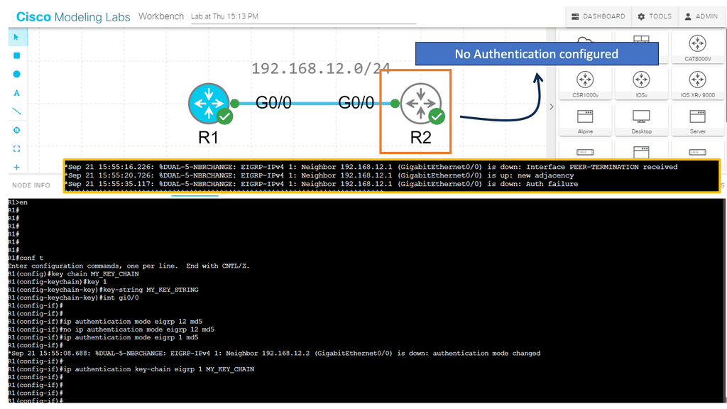
EIGRP authentication is a feature that adds an extra layer of security to network communication. It allows routers to validate the authenticity of the neighboring routers before exchanging routing information. By implementing EIGRP authentication, you can prevent unauthorized devices from participating in the routing process and ensure the integrity of your network.
Note:
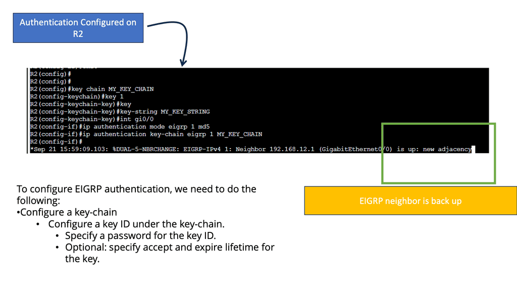
Two main components are required to implement EIGRP authentication: a key chain and an authentication algorithm. The key chain contains one or more keys, each with a unique key ID and a corresponding key string. The authentication algorithm, such as MD5 or SHA, generates a message digest based on the key string.
How does authentication benefit us?
- Every routing update packet you receive from your router will be authenticated.
- False routing updates from unapproved sources can be prevented.
- Malicious routing updates should be ignored.
A potential hacker could attempt the following things sitting on your network with a laptop:
- Advertise junk routes in your neighbor adjacency.
- Test whether you can drop the neighbor adjacency of one of your authorized routers by sending malicious packets.
Analysis:
To ensure the success of EIGRP authentication, it is crucial to follow some best practices. These include regularly changing passwords, using complex and unique shared secrets, enabling encryption for password transmission, and monitoring authentication logs for suspicious activity.
Conclusion: EIGRP authentication is an effective means of securing network communication within an enterprise environment. By implementing authentication mechanisms such as simple password authentication or message digest authentication, network administrators can mitigate the risk of unauthorized access and malicious routing information. Remember to carefully configure and manage authentication settings to maintain a robust and secure network infrastructure.
Route Summarization
Route summarization involves creating one summary route that represents multiple networks/subnets. Supernetting is also known as route aggregation.
There are several advantages to summarizing:
- Reduces memory requirements by shrinking routing tables.
- We save bandwidth by advertising fewer routes.
- Processing fewer packets and maintaining smaller routing tables saves CPU cycles.
- A flapping network can cause routing tables to become unstable.
Summarizing has some disadvantages as well:
- A router will drop traffic for unused networks without an appropriate destination in the routing table. The summary route may include networks not in use when we use summarization. Routers that have summary routes forward traffic to routers that advertise summary routes.
- The router prefers the path with the longest prefix match. When you use summaries, your router may choose another path where it has learned a more specific network. There is also a single metric for the summary route.
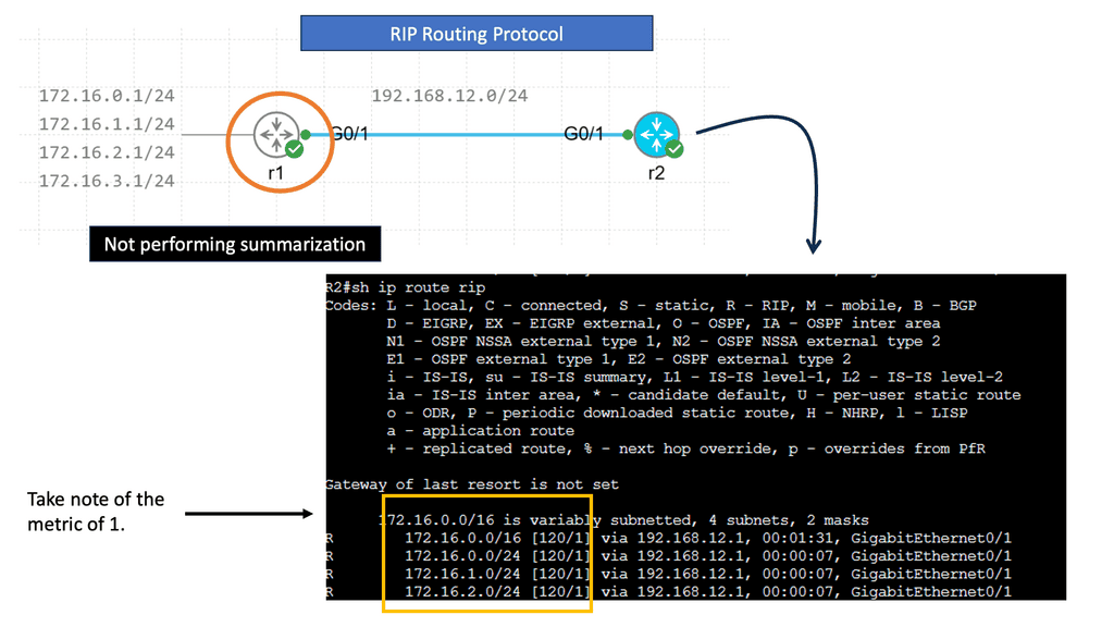
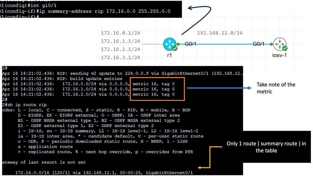
R1 advertises four different networks, and R2 receives them. The more information we advertise, the more bandwidth we require and the more CPU cycles we need to process. Of course, four networks on a Gigabit interface are no problem, but thousands or hundreds of networks are advertised in more extensive networks.
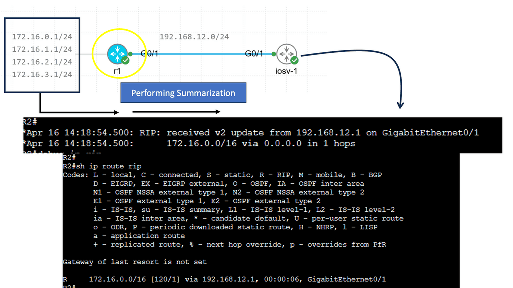
RIP creates a summary entry in the RIP routing database when a summary address is needed in the RIP database. Summary addresses remain in routing databases as long as there are child routes. In addition to removing the last child route, the summary entry is also removed from the database. Because each child route is not listed in an entry, this method of handling database entries reduces the number of entries in the database.
For RIP Version 2 route summarization, the lowest metric of an aggregated entry or the lowest metric of all current child routes must be advertised. For aggregated summarized routes, the best metric should be calculated at route initialization or when metric modifications are made to specific routes at the time of advertisement, not when the aggregated routes are advertised.
Administrative Distance
Suppose a network runs two routing protocols at once, OSPF and EIGRP. R1 receives information from both routing protocols.
- The router should send IP packets using the top path according to EIGRP.
- The router should use the bottom path to send IP packets in OSPF.
What routing information are we going to use? Which one? Do you use OSPF or EIGRP?
When two routing protocols provide information about the same destination network, we must make a choice. You can’t go left and right at the same time. We need to consider AD or administrative distance.
Administrative distance should be as low as possible. Directly connected routes have an AD of 0. Since nothing is better than directly connecting it to your router, it makes sense. Because static routes are configured manually, they have a shallow administrative distance of 1. You can sometimes override a routing protocol’s decision with a static route.
Since EIGRP is a Cisco routing protocol, its administrative distance is 90. RIP has 120, while OSPF has 110. Because EIGRP’s AD of 90 is lower than OSPF’s 110, we will use the information EIGRP tells us in the routing table.
**Closing Points: IP Forwarding**
IP forwarding is crucial in ensuring efficient and reliable data transmission in networking. As a fundamental component of network routing, IP forwarding enables packets of data to be forwarded from one network interface to another, ultimately reaching their intended destination. In this blog post, we delved deeper into IP forwarding, its significance, and its implementation in modern network infrastructures.
IP forwarding, or packet forwarding, refers to direct data packets from one network interface to another based on their destination IP addresses. It is the backbone of network routing, enabling seamless data flow across different networks. IP forwarding is typically performed by routers, specialized network devices designed to route packets between networks efficiently.
IP forwarding is essential in enabling effective communication between devices on different networks. By forwarding packets based on their destination IP addresses, IP forwarding allows data to traverse multiple networks, reaching its intended recipient. This capability is particularly critical in large-scale networks, such as the Internet, where data needs to travel through numerous routers before reaching its final destination.
Implementation of IP Forwarding:
Routers use routing tables to determine the best path for forwarding packets to implement IP forwarding. These routing tables contain a list of network destinations and associated next-hop router addresses. When a router receives a packet, it examines the destination IP address and consults its routing table to determine the appropriate next-hop router for forwarding the packet. This process continues until the packet reaches its final destination.
IP forwarding relies on routing protocols, such as Border Gateway Protocol (BGP) or Open Shortest Path First (OSPF), to exchange routing information between routers. These protocols enable routers to dynamically update their routing tables based on changing network conditions, ensuring packets are forwarded along the most optimal paths.
Key Points on Default Gateway
Default gateways are routers or multilayer switches (switches that can do routing) used by hosts to reach destinations outside their networks.
When it wants to send something to another host, a host checks whether the destination is within or outside its network. When in the same network, it uses address resolution protocol (ARP) to determine the destination’s MAC address and can then send IP packets. What is the host’s method for checking whether the destination belongs to the same network? Subnet masks are used for this purpose.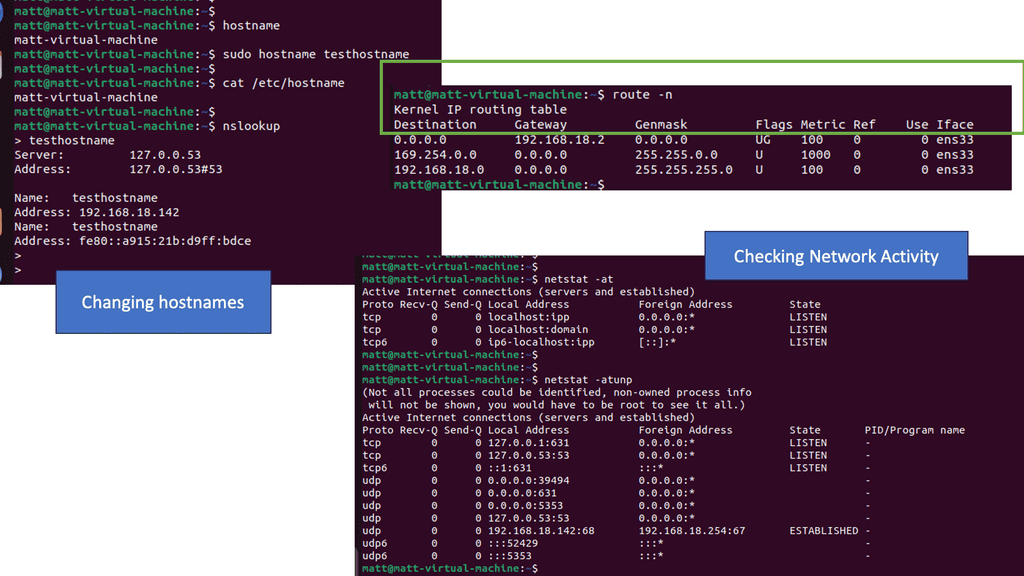
Analysis:
Netstat is a versatile utility used across different operating systems, including Windows, macOS, and Linux. It lets users view active network connections, monitor traffic, and troubleshoot network issues.
The netstat command generates displays that show network status and protocol statistics. You can display the status of TCP and UDP endpoints in table format, routing table information, and interface information.
Netstat offers a wide range of commands that can be utilized to gather specific information. Let’s take a look at some commonly used netstat commands:
- netstat -a: This command displays all active connections and listening ports on the system, providing valuable insights into network activities.
- netstat -r: This command lets users view the system’s routing table, which shows the paths that network traffic takes to reach its destination. This information is crucial for network troubleshooting and optimization.
- netstat -n: This command instructs netstat to display numerical IP addresses and port numbers instead of resolving them to hostnames. It can help identify network performance issues and potential security risks.
Advanced Netstat Techniques
Netstat goes beyond essential network monitoring. Here are a few advanced techniques that can further enhance its utility:
- netstat -p: This command allows users to view the specific process or application associated with each network connection. Administrators can identify potential bottlenecks and optimize system performance by knowing which processes utilize network resources.
- netstat -s: By using this command, users can access detailed statistics about various network protocols, including TCP, UDP, and ICMP. These statistics provide valuable insights into network utilization and can aid in troubleshooting network-related issues.
Closing Points: IP Forwarding
IP forwarding operates through a series of steps that involve examining packet headers, making routing decisions, and forwarding packets accordingly. When a data packet arrives at a router, the router checks the destination IP address within the packet header and consults its routing table. This table contains a list of routes that guide the packet to its final destination. Based on the routing table, the router determines the best path for the packet and forwards it to the next hop on its journey.
Routing protocols play a pivotal role in IP forwarding, as they update and maintain the routing tables that routers rely on. Protocols such as OSPF (Open Shortest Path First) and BGP (Border Gateway Protocol) enable routers to exchange information about network topology, ensuring that each router has the most accurate and efficient routes possible. These protocols help manage changes within the network, such as link failures or congestion, by dynamically adjusting routes to optimize data flow.
Despite its efficiency, IP forwarding faces several challenges, particularly in large-scale networks. Issues such as packet loss, latency, and network congestion can impact the performance of IP forwarding. Network administrators must continually monitor and optimize routing strategies to mitigate these challenges. Additionally, security concerns, such as IP spoofing and routing attacks, necessitate robust security measures to protect the integrity of data transmission.