Hello, I recently completed a 3 part package for Uniken. Part 1 can be found here – Matt Conran & Uniken. Stayed tuned for Part 2 and Part 3!

Paessler – NetFlow for Cybersecurity
Paessler purchased a three package article on NetFlow for Cybersecurity. Generally, the three posts relate to how NetFlow can be used to battle the ongoing threats of cybercriminals. Kindly, click the links. Part 1 – Matt Conran Paessler, Part 2 – Matt Conran Outbound DDoS, Part 3 – Matt Conran Cyberhunter.

Aviatrix Hybrid Cloud – Active Directory
Aviatrix, a hybrid cloud networking specialist used a 3 part blog package to formulate a solution brief – ActiveDirectoryTechBriefWhitePaperR1

Nominum Security Report
I had the pleasure to contribute to Nominum’s Security Report. Kindly click on the link to register and download – Matt Conran with Nominum
“Nominum Data Science just released a new Data Science and Security report that investigates the largest threats affecting organizations and individuals, including ransomware, DDoS, mobile device malware, IoT-based attacks and more. Below is an excerpt:
October 21, 2016, was a day many security professionals will remember. Internet users around the world couldn’t access their favorite sites like Twitter, Paypal, The New York Times, Box, Netflix, and Spotify, to name a few. The culprit: a massive Distributed Denial of Service (DDoS) attack against a managed Domain Name System (DNS) provider not well-known outside technology circles. We were quickly reminded how critical the DNS is to the internet as well as its vulnerability. Many theorize that this attack was merely a Proof of Concept, with far bigger attacks to come”

NS1 – Adding Intelligence to the Internet
I recently completed a two-part guest post for DNS-based company NS1. It discusses Internet challenges and introduces the NS1 traffic management solution – Pulsar. Part 1, kindly click – Matt Conran with NS1, and Part 2, kindly click – Matt Conran with NS1 Traffic Management.
“Application and service delivery over the public Internet is subject to various network performance challenges. This is because the Internet comprises different fabrics, connection points, and management entities, all of which are dynamic, creating unpredictable traffic paths and unreliable conditions. While there is an inherent lack of visibility into end-to-end performance metrics, for the most part, the Internet works, and packets eventually reach their final destination. In this post, we’ll discuss key challenges affecting application performance and examine the birth of new technologies,multi-CDNN designs, and how they affect DNS. Finally, we’ll look at Pulsar and our real-time telemetry engine developed specifically for overcoming many performance challenges by adding intelligence at the DNS lookup stage.”
SD WAN Tutorial: Nuage Networks

Nuage Networks
The following post details Nuage Netowrk and its response to SD-WAN. Part 2 can be found here with Nuage Network and SD-WAN. It’s a 24/7 connected world, and traffic diversity puts the Wide Area Network (WAN) edge to the test. Today’s applications should not be hindered by underlying network issues or a poorly designed WAN. Instead, the business requires designers to find a better way to manage the WAN by adding intelligence via an SD WAN Overlay with improved flow management, visibility, and control.
The WAN Monitoring role has changed from providing basic inter-site connectivity to adapting technology to meet business applications’ demands. It must proactively manage flows over all available paths, regardless of transport type. Business requirements should drive today’s networks, and the business should dictate the directions of flows, not the limitations of a routing protocol. The remainder of the post relates to Nuage Network and services as a good foundation for an SD WAN tutorial.
For additional information, you may find the following posts helpful:
Nuage SD WAN. |
|
The building blocks of the WAN have remained stagnant while the application environment has dynamically shifted; sure, speeds and feeds have increased, but the same architectural choices that were best practice 10 or 15 years ago are still being applied, hindering rapid growth in business evolution. So how will the traditional WAN edge keep up with new application requirements?
Nuage SD WAN
Nuage Networks SD-WAN solution challenges this space and overcomes existing WAN limitations by bringing intelligence to routing at an application level. Now, policy decisions are made by a central platform that has full WAN and data center visibility. A transport-agnostic WAN optimizes the network and the decisions you make about it. In the eyes of Nuage, “every packet counts,” and mission-critical applications are always available on protected premium paths.
Routing Protocols at the WAN Edge
Routing protocols assist in the forwarding decisions for traffic based on destinations, with decisions made hop-by-hop. This limits the number of paths the application traffic can take. Paths are further limited to routing loop restrictions – routing protocols will not take a path that could potentially result in a forwarding loop. Couple this with the traditional forwarding paradigms of primitive WAN designs, resulting in a network that cannot match today’s application requirements. We need to find more granular ways to forward traffic.
There has always been a problem with complex routing for the WAN. BGP supports the best path, and ECMP provides some options for path selection. Solutions like Dynamic Multipoint VPN (DMVPN) operate with multiple control planes that are hard to design and operate. It’s painful to configure QOS policies per-link basis and design WAN solutions to incorporate multiple failure scenarios. The WAN is the most complex module of any network yet so important as it acts as the gateway to other networks such as the branch LAN and data center.
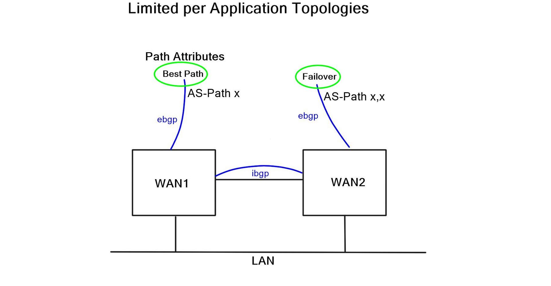
Best path & failover only.
At the network edge, where there are two possible exit paths, choosing a path based on a unique business characteristic is often desirable. For example, use a historical jitter link for web traffic or premium links for mission-critical applications. The granularity for exit path selection should be flexible and selected based on business and application requirements. Criteria for exit points should be application-independent, allowing end-to-end network segmentation.
External policy-based protocol
BGP is an external policy-based protocol commonly used to control path selection. BGP peers with other BGP routers to exchange Network Layer Reachability Information (NLRI). Its flexible policy-orientated approach and outbound traffic engineering offer tailored control for that network slice. As a result, it offers more control than an Interior Gateway Protocol (IGP) and reduces network complexity in large networks. These factors have made BGP the de facto WAN edge routing protocol.
However, the path attributes that influence BGP does not consider any specifically tailored characteristics, such as unique metrics, transit performance, or transit brownouts. When BGP receives multiple paths to the same destination, it runs the best path algorithm to decide the best path to install in the IP routing table; generally, this path selection is based on AS-Path. Unfortunately, AS-Path is not an efficient measure of end-to-end transit. It misses the shape of the network, which can result in long path selection or paths experiencing packet loss.
The traditional WAN
Traditional WAN routes down one path and, by default, have no awareness of what’s happening at the application level (packet loss, jitter, retransmissions). There have been many attempts to enhance the WANs behavior. For example, SLA steering based on enhanced object tracking would poll a metric such as Round Trip Time (RTT).
These methods are popular and widely implemented, but failover events occur on a configurable metric. All these extra configuration parameters make the WAN more complex. Simply acting as band-aids for a network that is under increasing pressure.
“Nuage Networks sponsor this post. All thoughts and opinions expressed are the authors.”

DMVPN Phases | DMVPN Phase 1 2 3
Highlighting DMVPN Phase 1 2 3
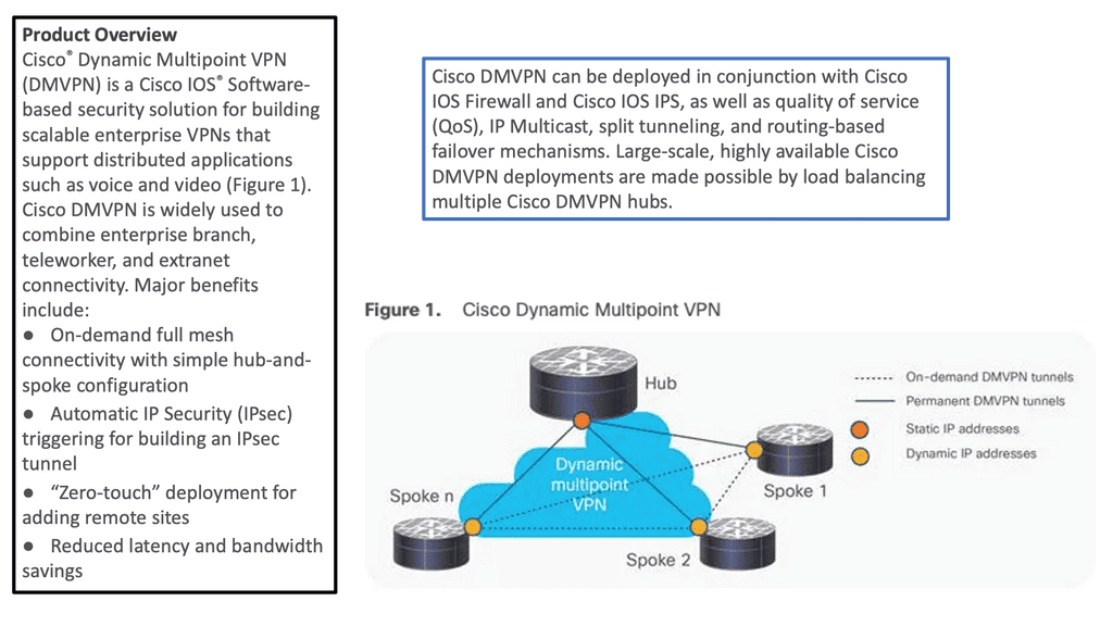
Dynamic Multipoint Virtual Private Network ( DMVPN ) is a dynamic virtual private network ( VPN ) form that allows a mesh of VPNs without needing to pre-configure all tunnel endpoints, i.e., spokes. Tunnels on spokes establish on-demand based on traffic patterns without repeated configuration on hubs or spokes. The design is based on DMVPN Phase 1 2 3.
- Point-to-multipoint Layer 3 overlay VPN
In its simplest form, DMVPN is a point-to-multipoint Layer 3 overlay VPN enabling logical hub and spoke topology supporting direct spoke-to-spoke communications depending on DMVPN design ( DMVPN Phases: Phase 1, Phase 2, and Phase 3 ) selection. The DMVPN Phase selection significantly affects routing protocol configuration and how it works over the logical topology. However, parallels between frame-relay routing and DMVPN routing protocols are evident from a routing point of view.
- Dynamic routing capabilities
DMVPN is one of the most scalable technologies when building large IPsec-based VPN networks with dynamic routing functionality. It seems simple, but you could encounter interesting design challenges when your deployment has more than a few spoke routers. This post will help you understand the DMVPN phases and their configurations.
DMVPN Phases. |
|
DMVPN allows the creation of full mesh GRE or IPsec tunnels with a simple template of configuration. From a provisioning point of view, DMPVN is simple.
Before you proceed, you may find the following useful:
- A key point: Video on the DMVPN Phases
The following video discusses the DMVPN phases. The demonstration is performed with Cisco modeling labs, and I go through a few different types of topologies. At the same time, I was comparing the configurations for DMVPN Phase 1 and DMVPN Phase 3. There is also some on-the-fly troubleshooting that you will find helpful and deepen your understanding of DMVPN.

Back to basics with DMVPN.
- Highlighting DMVPN
DMVPN is a Cisco solution providing scalable VPN architecture. In its simplest form, DMVPN is a point-to-multipoint Layer 3 overlay VPN enabling logical hub and spoke topology supporting direct spoke-to-spoke communications depending on DMVPN design ( DMVPN Phases: Phase 1, Phase 2, and Phase 3 ) selection. The DMVPN Phase selection significantly affects routing protocol configuration and how it works over the logical topology. However, parallels between frame-relay routing and DMVPN routing protocols are evident from a routing point of view.
- Introduction to DMVPN technologies
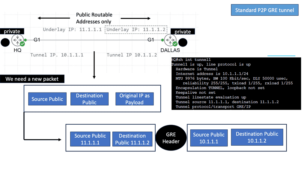
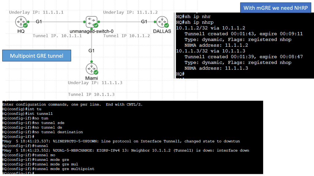
DMVPN uses industry-standardized technologies ( NHRP, GRE, and IPsec ) to build the overlay network. DMVPN uses Generic Routing Encapsulation (GRE) for tunneling, Next Hop Resolution Protocol (NHRP) for on-demand forwarding and mapping information, and IPsec to provide a secure overlay network to address the deficiencies of site-to-site VPN tunnels while providing full-mesh connectivity.
In particular, DMVPN uses Multipoint GRE (mGRE) encapsulation and supports dynamic routing protocols, eliminating many other support issues associated with other VPN technologies. The DMVPN network is classified as an overlay network because the GRE tunnels are built on top of existing transports, also known as an underlay network.
DMVPN Is a Combination of 4 Technologies:
mGRE: In concept, GRE tunnels behave like point-to-point serial links. mGRE behaves like LAN, so many neighbors are reachable over the same interface. The “M” in mGRE stands for multipoint.
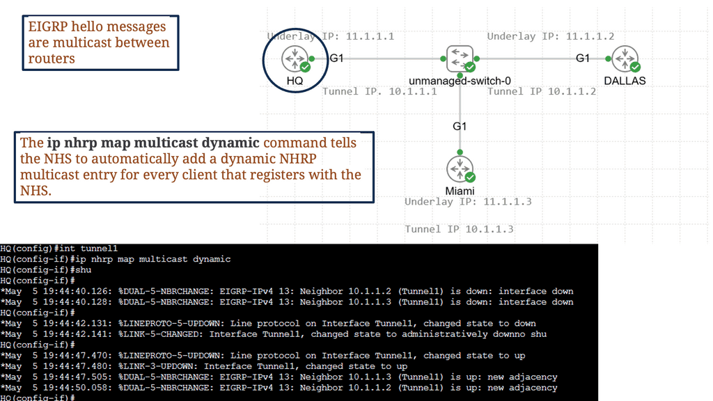
Dynamic Next Hop Resolution Protocol ( NHRP ) with Next Hop Server ( NHS ): LAN environments utilize Address Resolution Protocol ( ARP ) to determine the MAC address of your neighbor ( inverse ARP for frame relay ). mGRE, the role of ARP is replaced by NHRP. NHRP binds the logical IP address on the tunnel with the physical IP address used on the outgoing link ( tunnel source ).
The resolution process determines if you want to form a tunnel destination to X and what address tunnel X resolve towards. DMVPN binds IP-to-IP instead of ARP, which binds destination IP to destination MAC address.
- A key point: Lab guide on Next Hop Resolution Protocol (NHRP)
So we know that NHRP is a dynamic routing protocol that focuses on resolving the next hop address for packet forwarding in a network. Unlike traditional static routing protocols, DNHRP adapts to changing network conditions and dynamically determines the optimal path for data transmission. It works with a client-server model. The DMVPN hub is the NHS, and the Spokes are the NHC.
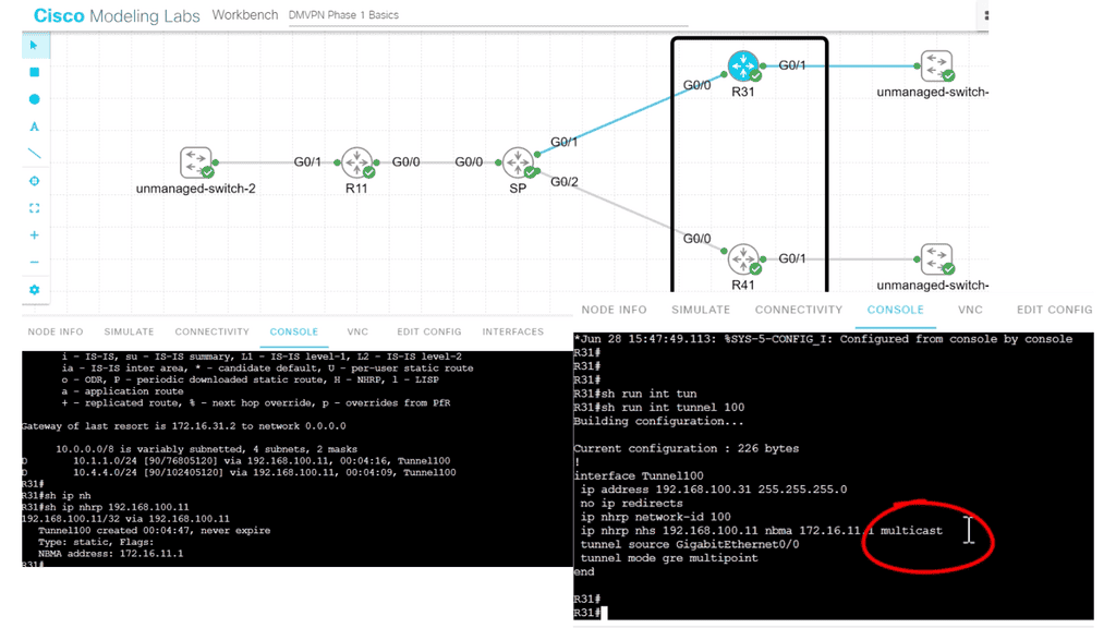
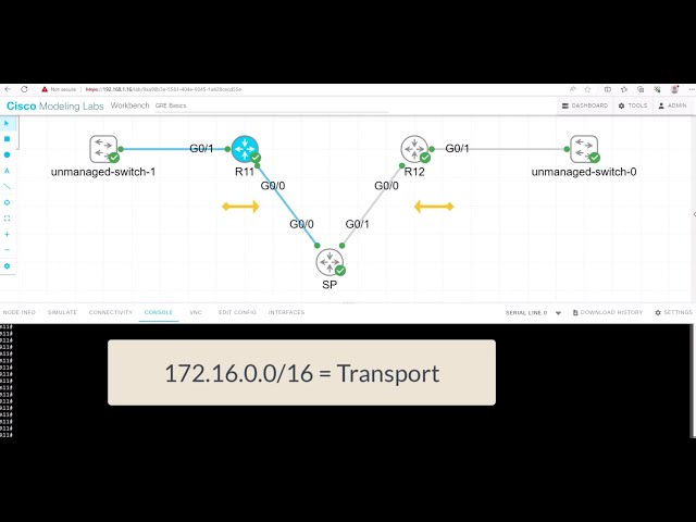
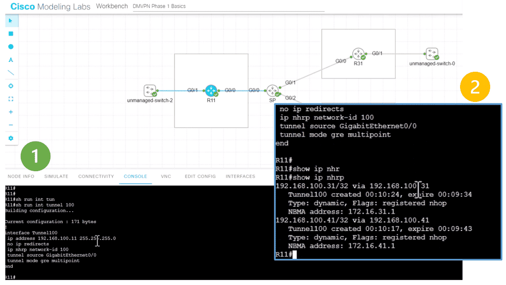
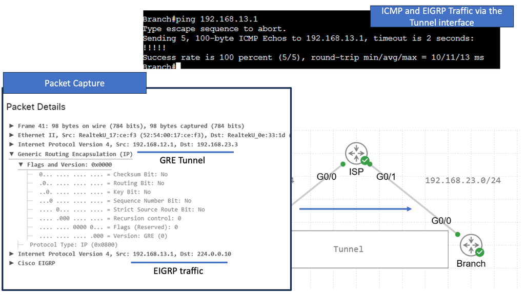
In the following lab topology, we have R11 as the hub with two spokes, R31 and R41. The spokes need to explicitly configure the next hop server (NHS) information with the command: IP nhrp NHS 192.168.100.11 nbma 172.16.11.1. Notice we have the “multicast” keyword at the end of the configuration line. This is used to allow multicast traffic.
As the routing protocol over the DMVPN tunnel, I am running EIGRP, which requires multicast Hellos to form EIGRP neighbor relationships. To form neighbor relationships with BGP, you use TCP, so you would not need the “multicast” keyword.
IPsec tunnel protection and IPsec fault tolerance: DMVPN is a routing technique not directly related to encryption. IPsec is optional and used primarily over public networks. Potential designs exist for DMVPN in public networks with GETVPN, which allows the grouping of tunnels to a single Security Association ( SA ).
Routing: Designers are implementing DMVPN without IPsec for MPLS-based networks to improve convergence as DMVPN acts independently of service provider routing policy. The sites only need IP connectivity to each other to form a DMVPN network. It would be best to ping the tunnel endpoints and route IP between the sites. End customers decide on the routing policy, not the service provider, offering more flexibility than sites connected by MPLS. MPLS-connected sites, the service provider determines routing protocol policies.
Map IP to IP: If you want to reach my private address, you need to GRE encapsulate it and send it to my public address. Spoke registration process.
DMVPN Phases Explained
DMVPN Phases: DMVPN phase 1 2 3
The DMVPN phase selected influence spoke-to-spoke traffic patterns supported routing designs and scalability.
- DMVPN Phase 1: All traffic flows through the hub. The hub is used in the network’s control and data plane paths.
- DMVPN Phase 2: Allows spoke-to-spoke tunnels. Spoke-to-spoke communication does not need the hub in the actual data plane. Spoke-to-spoke tunnels are on-demand based on spoke traffic triggering the tunnel. Routing protocol design limitations exist. The hub is used for the control plane but, unlike phase 1, not necessarily in the data plane.
- DMVPN Phase 3: Improves scalability of Phase 2. We can use any Routing Protocol with any setup. “NHRP redirects” and “shortcuts” take care of traffic flows.
- A key point: Video on DMVPN
In the following video, we will start with the core block of DMVPN, GRE. Generic Routing Encapsulation (GRE) is a tunneling protocol developed by Cisco Systems that can encapsulate a wide variety of network layer protocols inside virtual point-to-point links or point-to-multipoint links over an Internet Protocol network.
We will then move to add the DMVPN configuration parameters. Depending on the DMVPN phase you want to implement, DMVPN can be enabled with just a few commands. Obviously, it would help if you had the underlay in place.
As you know, DMVPN operates as the overlay that lays up an existing underlay network. This demonstration will go through DMVPN Phase 1, which was the starting point of DMVPN, and we will touch on DMVPN Phase 3. We will look at the various DMVPN and NHRP configuration parameters along with the show commands.
The DMVPN Phases
DMVPN Phase 1
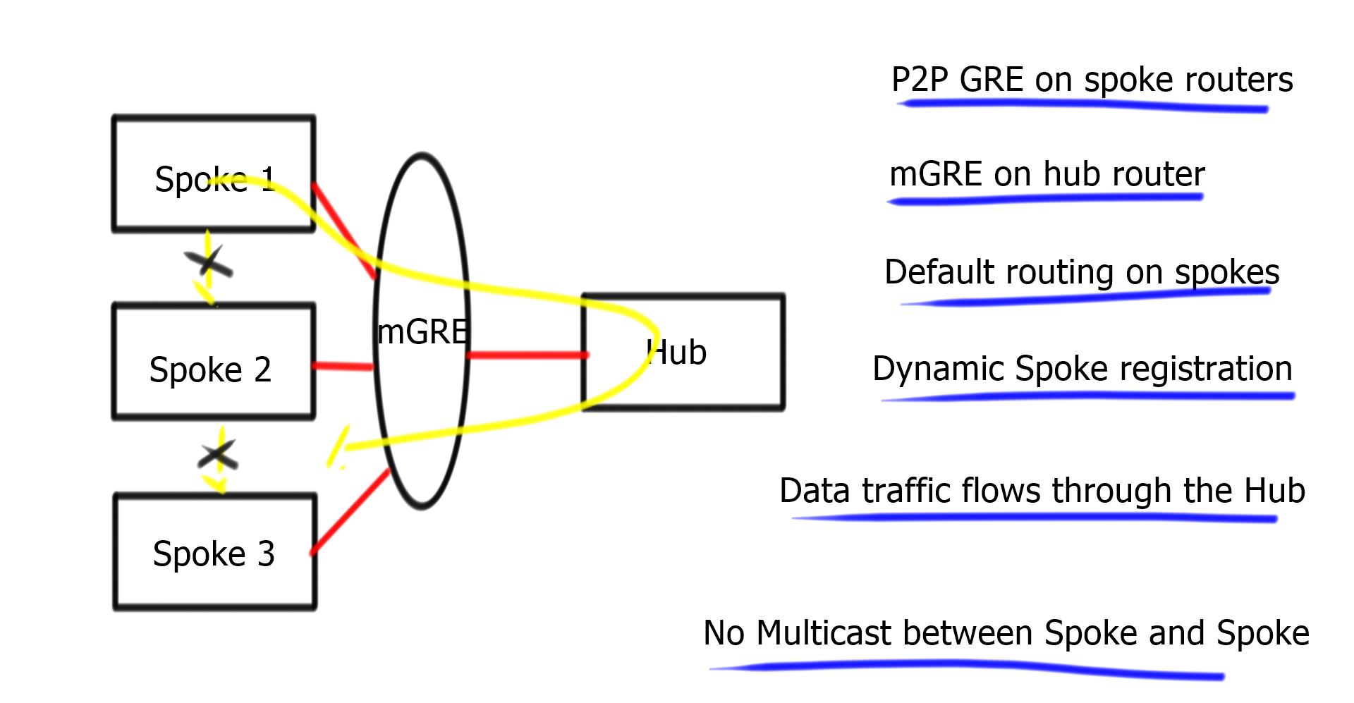
- Phase 1 consists of mGRE on the hub and point-to-point GRE tunnels on the spoke.
Hub can reach any spoke over the tunnel interface, but spokes can only go through the hub. No direct Spoke-to-Spoke. Spoke only needs to reach the hub, so a host route to the hub is required. Perfect for default route design from the hub. Design against any routing protocol, as long as you set the next hop to the hub device.
Multicast ( routing protocol control plane ) exchanged between the hub and spoke and not spoke-to-spoke.
On spoke, enter adjust MMS to help with environments where Path MTU is broken. It must be 40 bytes lower than the MTU – IP MTU 1400 & IP TCP adjust-mss 1360. In addition, it inserts the max segment size option in TCP SYN packets, so even if Path MTU does not work, at least TCP sessions are unaffected.
- A key point: Tunnel keys
Tunnel keys are optional for hubs with a single tunnel interface. They can be used for parallel tunnels, usually in conjunction with VRF-light designs. Two tunnels between the hub and spoke, the hub cannot determine which tunnel it belongs to based on destination or source IP address. Tunnel keys identify tunnels and help map incoming GRE packets to multiple tunnel interfaces.

Tunnel Keys on 6500 and 7600: Hardware cannot use tunnel keys. It cannot look that deep in the packet. The CPU switches all incoming traffic, so performance goes down by 100. You should use a different source for each parallel tunnel to overcome this. If you have a static configuration and the network is stable, you could use a “hold-time” and “registration timeout” based on hours, not the 60-second default.
In carrier Ethernet and Cable networks, the spoke IP is assigned by DHCP and can change regularly. Also, in xDSL environments, PPPoE sessions can be cleared, and spokes get a new IP address. Therefore, non-Unique NHRP Registration works efficiently here.
Routing Protocol
Routing for Phase 1 is simple. Summarization and default routing at the hub are allowed. The hub constantly changes next-hop on spokes; the hub is always the next hop. Spoke needs to first communicate with the hub; sending them all the routing information makes no sense. So instead, send them a default route.
Careful with recursive routing – sometimes, the Spoke can advertise its physical address over the tunnel. Hence, the hub attempts to send a DMVPN packet to the spoke via the tunnel, resulting in tunnel flaps.
DMVPN phase 1 OSPF routing
Recommended design should use different routing protocols over DMVPN, but you can extend the OSPF domain by adding the DMVPN network into a separate OSPF Area. Possible to have one big area but with a large number of spokes; try to minimize the topology information spokes have to process.
Redundant set-up with spoke running two tunnels to redundant Hubs, i.e., Tunnel 1 to Hub 1 and Tunnel 2 to Hub 2—designed to have the tunnel interfaces in the same non-backbone area. Having them in separate areas will cause spoke to become Area Border Router ( ABR ). Every OSPF ABR must have a link to Area 0. Resulting in complex OSPF Virtual-Link configuration and additional unnecessary Shortest Path First ( SPF ) runs.
Make sure the SPF algorithm does not consume too much spoke resource. If Spoke is a high-end router with a good CPU, you do not care about SPF running on Spoke. Usually, they are low-end routers, and maintaining efficient resource levels is critical. Potentially design the DMVPN area as a stub or totally stub area. This design prevents changes (for example, prefix additions ) on the non-DVMPN part from causing full or partial SPFs.
Low-end spoke routers can handle 50 routers in single OSPF area.
Configure OSPF point-to-multipoint. Mandatory on the hub and recommended on the spoke. Spoke has GRE tunnels, by default, use OSPF point-to-point network type. Timers need to match for OSPF adjacency to come up.
OSPF is hierarchical by design and not scalable. OSPF over DMVPN is fine if you have fewer spoke sites, i.e., below 100.
DMVPN phase 1 EIGRP routing
On the hub, disable split horizon and perform summarization. Then, deploy EIGRP leak maps for redundant remote sites. Two routers connecting the DMVPN and leak maps specify which information ( routes ) can leak to each redundant spoke.
Deploy spokes as Stub routers. Without stub routing, whenever a change occurs ( prefix lost ), the hub will query all spokes for path information.
Essential to specify interface Bandwidth.
- A key point: Lab guide with DMVPN phase 1 EIGRP.
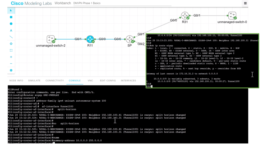
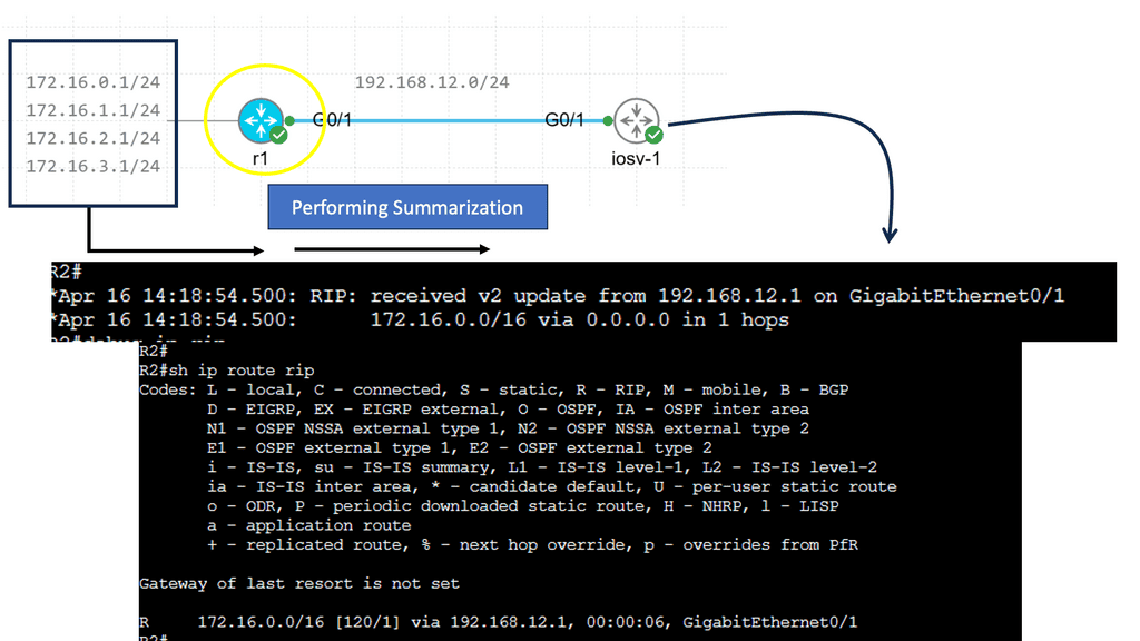
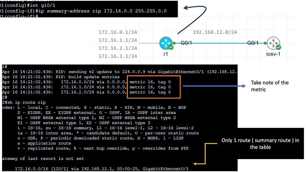
In the following lab guide, I show how to turn on and off split horizon at the hub sites, R11. So when you turn on split-horizon, the spokes will only see the routes behind R11; in this case, it’s actually only one route. They will not see routes from the other spokes. In addition, I have performed summarization on the hub site. Notice how the spoke only see the summary route.
Turning the split horizon on with summarization, too, will not affect spoke reachability as the hub summarizes the routes. So, if you are performing summarization at the hub site, you can also have split horizon turned on at the hub site, R11,
DMVPN phase 1 BGP routing
Recommended using EBGP. Hub must have next-hop-self on all BGP neighbors. To save resources and configuration steps, possible to use policy templates. Avoid routing updates to spokes by filtering BGP updates or advertising the default route to spoke devices.
In recent IOS, we have dynamic BGP neighbors. Configure the range on the hub with command BGP listens to range 192.168.0.0/24 peer-group spokes. Inbound BGP sessions are accepted if the source IP address is in the specified range of 192.168.0.0/24.
DMVPN Phase 2
Phase 2 allowed mGRE on the hub and spoke, permitting spoke-to-spoke on-demand tunnels. Phase 2 consists of no changes on the hub router; change tunnel mode on spokes to GRE multipoint – tunnel mode gre multipoint. Tunnel keys are mandatory when multiple tunnels share the same source interface.
Multicast traffic still flows between the hub and spoke only, but data traffic can now flow from spoke to spoke.
DMVPN Packet Flows and Routing
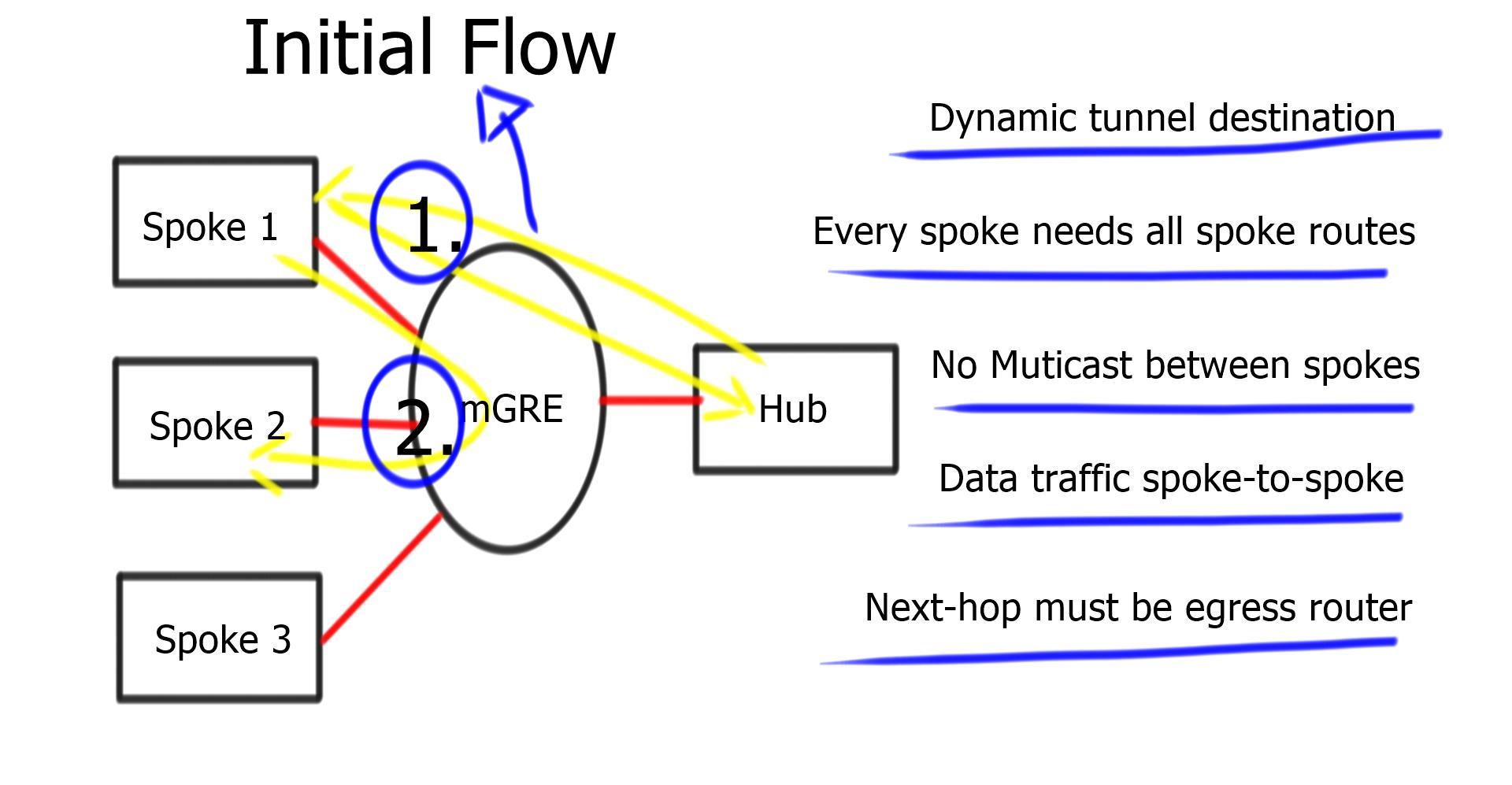
DMVPN phase 2 packet flow
| -For initial packet flow, even though the routing table displays the spoke as the Next Hop, all packets are sent to the hub router. Shortcut not established. |
| -The spokes send NHRP requests to the Hub and ask the hub about the IP address of the other spokes. |
| -Reply is received and stored on the NHRP dynamic cache on the spoke router. |
| -Now, spokes attempt to set up IPSEC and IKE sessions with other spokes directly. |
| -Once IKE and IPSEC become operational, the NHRP entry is also operational, and the CEF table is modified so spokes can send traffic directly to spokes. |
The process is unidirectional. Reverse traffic from other spoke triggers the exact mechanism. Spokes don’t establish two unidirectional IPsec sessions; Only one.
There are more routing protocol restrictions with Phase 2 than DMVPN Phases 1 and 3. For example, summarization and default routing is NOT allowed at the hub, and the hub always preserves the next hop on spokes. Spokes need specific routes to each other networks.
DMVPN phase 2 OSPF routing
Recommended using OSPF network type Broadcast. Ensure the hub is DR. You will have a disaster if a spoke becomes a Designated Router ( DR ). For that reason, set the spoke OSPF priority to “ZERO.”
OSPF multicast packets are delivered to the hub only. Due to configured static or dynamic NHRP multicast maps, OSPF neighbor relationships only formed between the hub and spoke.
The spoke router needs all routes from all other spokes, so default routing is impossible for the hub.
DMVPN phase 2 EIGRP routing
No changes to the spoke. Add no IP next-hop-self on a hub only—Disable EIRP split-horizon on hub routers to propagate updates between spokes.
Do not use summarization; if you configure summarization on spokes, routes will not arrive in other spokes. Resulting in spoke-to-spoke traffic going to the hub.
DMVPN phase 2 BGP pouting
Remove the next-hop-self on hub routers.
Split default routing
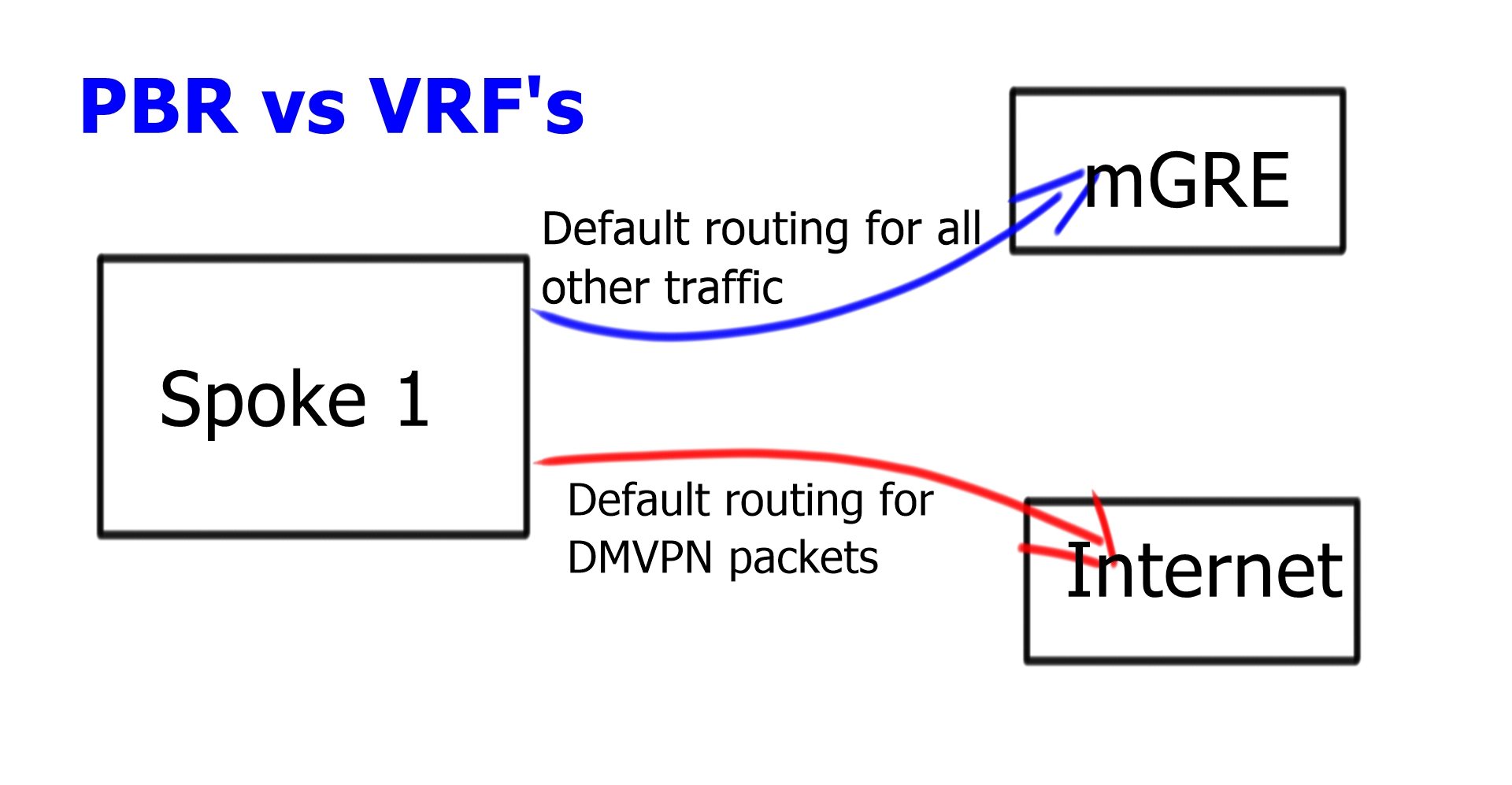
Split default routing may be used if you have the requirement for default routing to the hub: maybe for central firewall design, and you want all traffic to go there before proceeding to the Internet. However, the problem with Phase 2 allows spoke-to-spoke traffic, so even though we would default route pointing to the hub, we need the default route point to the Internet.
Require two routing perspectives; one for GRE and IPsec packets and another for data traversing the enterprise WAN. Possible to configure Policy Based Routing ( PBR ) but only as a temporary measure. PBR can run into bugs and is difficult to troubleshoot. Split routing with VRF is much cleaner. Routing tables for different VRFs may contain default routes. Routing in one VRF will not affect routing in another VRF.
Multi-homed remote site
To make it complicated, the spoke needs two 0.0.0/0. One for each DMVPN Hub network. Now, we have two default routes in the same INTERNET VRF. We need a mechanism to tell us which one to use and for which DMVPN cloud.

Even if the tunnel source is for mGRE-B ISP-B, the routing table could send the traffic to ISP-A. ISP-A may perform uRFC to prevent address spoofing. It results in packet drops.
The problem is that the outgoing link ( ISP-A ) selection depends on Cisco Express Forwarding ( CEF ) hashing, which you cannot influence. So, we have a problem: the outgoing packet has to use the correct outgoing link based on the source and not the destination IP address. The solution is Tunnel Route-via – Policy routing for GRE. To get this to work with IPsec, install two VRFs for each ISP.
DMVPN Phase 3

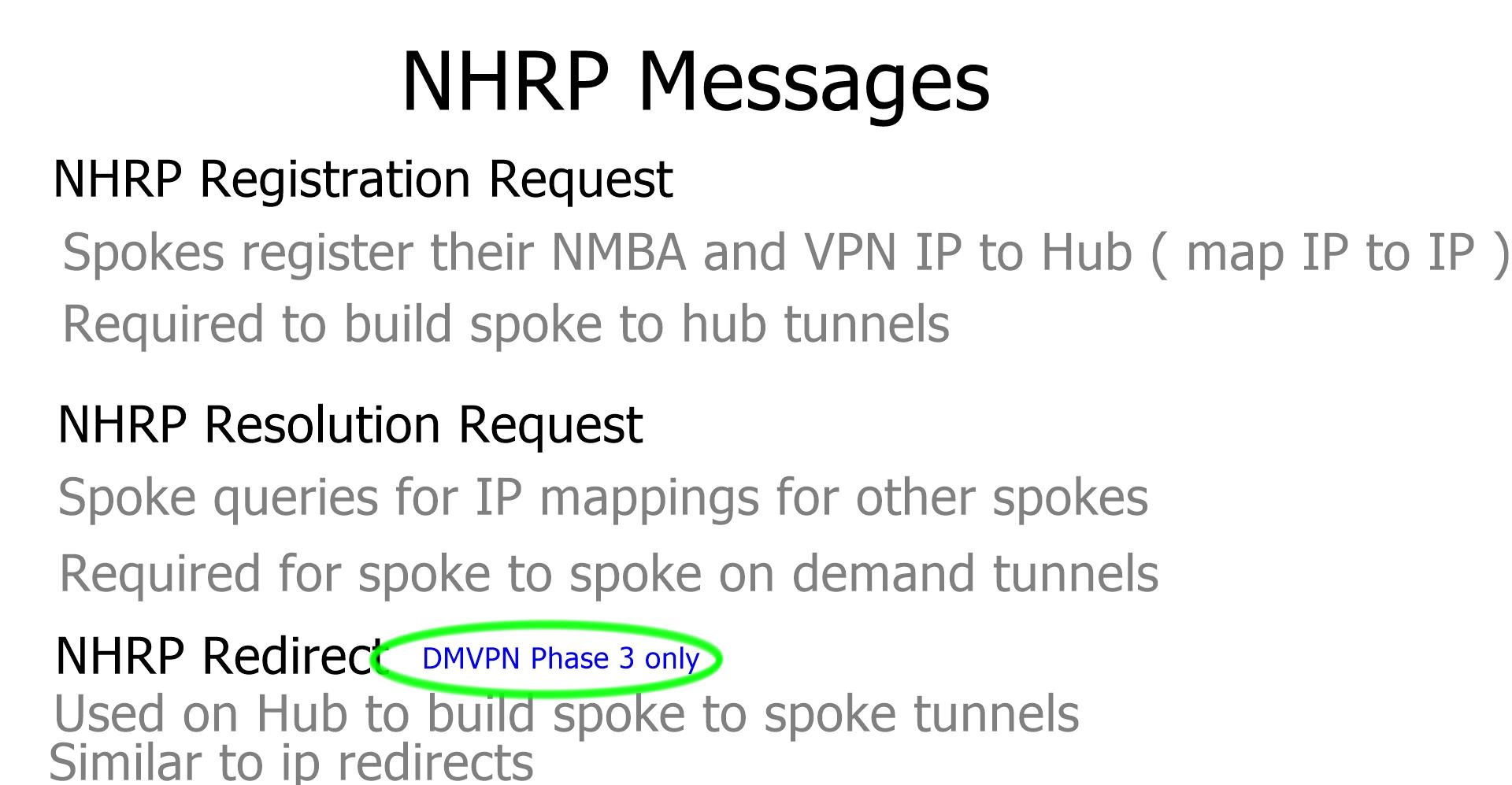
Phase 3 consists of mGRE on the hub and mGRE tunnels on the spoke. Allows spoke-to-spoke on-demand tunnels. The difference is that when the hub receives an NHRP request, it can redirect the remote spoke to tell them to update their routing table.
- A key point: Lab on DMVPN Phase 3 configuration
The following lab configuration shows an example of DMVPN Phase 3. The command: Tunnel mode gre multipoint GRE is on both the hub and the spokes. This contrasts with DMVPN Phase 1, where we must explicitly configure the tunnel destination on the spokes. Notice the command: Show IP nhrp. We have two spokes. dynamically learned via the NHRP resolution process with the flag “registered nhop.” However, this is only part of the picture for DMVPN Phase 3. We need configurations to enable dynamic spoke-to-spoke tunnels, and this is discussed next.
Phase 3 redirect features
The Phase 3 DMVPN configuration for the hub router adds the interface parameter command ip nhrp redirect on the hub router. This command checks the flow of packets on the tunnel interface and sends a redirect message to the source spoke router when it detects packets hair pinning out of the DMVPN cloud.
Hairpinning means traffic is received and sent to an interface in the same cloud (identified by the NHRP network ID). For instance, hair pinning occurs when packets come in and go out of the same tunnel interface. The Phase 3 DMVPN configuration for spoke routers uses the mGRE tunnel interface and the command ip nhrp shortcut on the tunnel interface.
Note: Placing ip nhrp shortcut and ip nhrp redirect on the same DMVPN tunnel interface has no adverse effects.
Phase 3 allows spoke-to-spoke communication even with default routing. So even though the routing table points to the hub, the traffic flows between spokes. No limits on routing; we still get spoke-to-spoke traffic flow even when you use default routes.
“Traffic-driven-redirect”; hub notices the spoke is sending data to it, and it sends a redirect back to the spoke, saying use this other spoke. Redirect informs the sender of a better path. The spoke will install this shortcut and initiate IPsec with another spoke. Use ip nhrp redirect on hub routers & ip nhrp shortcuts on spoke routers.
No restrictions on routing protocol or which routes are received by spokes. Summarization and default routing is allowed. The next hop is always the hub.
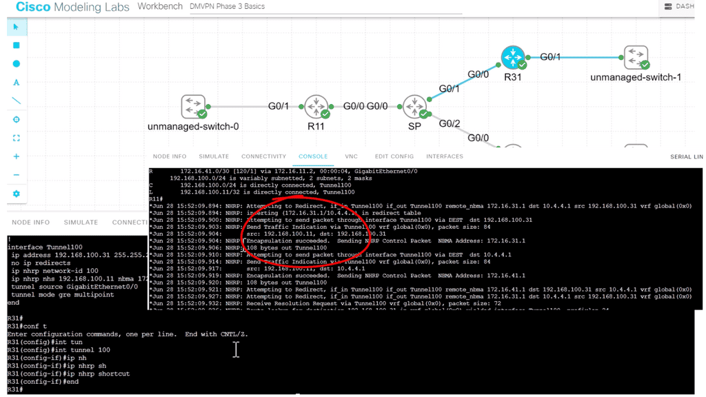
- A key point: Lab guide on DMVPN Phase 3
I have the command in the following lab guide: IP nhrp shortcut on the spoke, R31. I also have the “redirect” command on the hub, R11. So, we don’t see the actual command on the hub, but we do see that R11 is sending a “Traffic Indication” message to the spokes. This was sent when spoke-to-spoke traffic is initiated, informing the spokes that a better and more optimal path exists without going to the hub.
 | Main Checklist Points To Consider
|
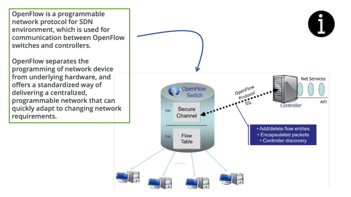
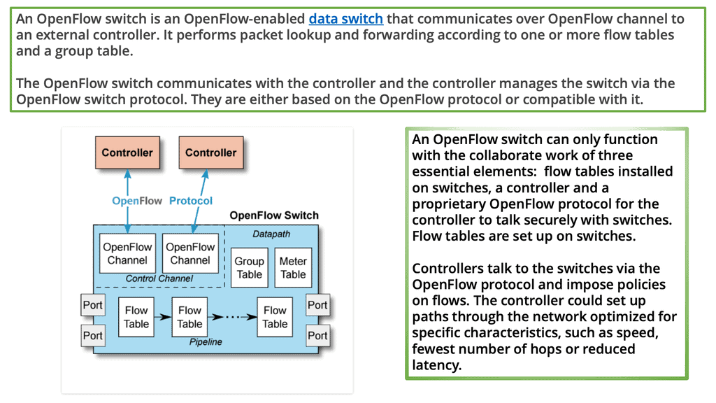
What is OpenFlow
How does OpenFlow work?
1: OpenFlow allows network controllers to determine the path of network packets in a network of switches. There is a difference between switches and controllers. With separate control and forwarding, traffic management can be more sophisticated than access control lists (ACLs) and routing protocols.
2: An OpenFlow protocol allows switches from different vendors, often with proprietary interfaces and scripting languages, to be managed remotely. Software-defined networking (SDN) is considered to be enabled by OpenFlow by its inventors.
3: With OpenFlow, Layer 3 switches can add, modify, and remove packet-matching rules and actions remotely. By doing so, routing decisions can be made periodically or ad hoc by the controller and translated into rules and actions with a configurable lifespan, which are then deployed to the switch’s flow table, where packets are forwarded at wire speed for the duration of the rule.
The Role of OpenFlow Controllers
If the switch cannot match packets, they can be sent to the controller. The controller can modify existing flow table rules or deploy new rules to prevent a structural traffic flow. It may even forward the traffic itself if the switch is instructed to forward packets rather than just their headers.
OpenFlow uses Transport Layer Security (TLS) over Transmission Control Protocol (TCP). Switches wishing to connect should listen on TCP port 6653. In earlier versions of OpenFlow, port 6633 was unofficially used. The protocol is mainly used between switches and controllers.
### Origins of OpenFlow
The inception of OpenFlow can be traced back to the early 2000s when researchers at Stanford University sought to create a more versatile and programmable network architecture. Traditional networking relied heavily on static and proprietary hardware configurations, which limited innovation and adaptability. OpenFlow emerged as a solution to these challenges, offering a standardized protocol that decouples the network control plane from the data plane. This separation allows for centralized control and dynamic adjustment of network traffic, fostering innovation and agility in network design.
### How OpenFlow Works
At its core, the OpenFlow protocol facilitates communication between network devices and a centralized SDN controller. It does this by using a series of flow tables within network switches, which are programmed by the controller. These flow tables dictate how packets should be handled, whether they are forwarded to a destination, dropped, or modified in some way. By leveraging OpenFlow, network administrators can deploy updates, optimize performance, and troubleshoot issues with unprecedented speed and precision, all from a single point of control.
Introducing SDN
Recent changes and requirements have driven networks and network services to become more flexible, virtualization-aware, and API-driven. One major trend affecting the future of networking is software-defined networking ( SDN ). The software-defined architecture aims to extract the entire network into a single switch.
Software-defined networking (SDN) is an evolving technology defined by the Open Networking Foundation ( ONF ). It involves the physical separation of the network control plane from the forwarding plane, where a control plane controls several devices. This differs significantly from traditional IP forwarding that you may have used in the past.
The Core Concepts of SDN
At its heart, Software-Defined Networking decouples the network control plane from the data plane, allowing network administrators to manage network services through abstraction of lower-level functionality. This separation enables centralized network control, which simplifies the management of complex networks. The control plane makes decisions about where traffic is sent, while the data plane forwards traffic to the selected destination. This approach allows for a more flexible, adaptable network infrastructure.
The activities around OpenFlow
Even though OpenFlow has received a lot of industry attention, programmable networks and decoupled control planes (control logic) from data planes have been around for many years. To enhance ATM, Internet, and mobile networks’ openness, extensibility, and programmability, the Open Signaling (OPENING) working group held workshops in 1995. A working group within the Internet Engineering Task Force (IETF) developed GSMP to control label switches based on these ideas. June 2002 marked the official end of this group, and GSMPv3 was published.
Data and control plane
Therefore, SDN separates the data and control plane. The main driving body behind software-defined networking (SDN) is the Open Networking Foundation ( ONF ). Introduced in 2008, the ONF is a non-profit organization that wants to provide an alternative to proprietary solutions that limit flexibility and create vendor lock-in.
The insertion of the ONF allowed its members to run proof of concepts on heterogeneous networking devices without requiring vendors to expose their software’s internal code. This creates a path for an open-source approach to networking and policy-based controllers.
Knowledge Check: Data & Control Plane
### Data Plane: The Highway for Your Data
The data plane, often referred to as the forwarding plane, is responsible for the actual movement of packets of data from source to destination. Imagine it as a network’s highway, where data travels at high speed. This component operates at the speed of light, handling massive amounts of data with minimal delay. It’s designed to process packets quickly, ensuring that the information arrives where it needs to be without interruption.
### Control Plane: The Brain Behind the Operation
While the data plane acts as the highway, the control plane is the brain that orchestrates the flow of traffic. It makes decisions about routing, managing the network topology, and controlling the data plane’s operations. The control plane uses protocols to determine the best paths for data and to update routing tables as needed. It’s responsible for ensuring that the network operates efficiently, adapting to changes, and maintaining optimal performance.
### Interplay Between Data and Control Planes
The synergy between the data and control planes is what enables modern networks to function effectively. The control plane provides the intelligence and decision-making necessary to guide the data plane. This interaction ensures that data packets take the best possible paths, reducing latency and maximizing throughput. As networks evolve, the lines between these planes may blur, but their distinct roles remain pivotal.
### Real-World Applications and Innovations
The concepts of data and control planes are not just theoretical—they have practical applications in technologies such as Software-Defined Networking (SDN) and Network Function Virtualization (NFV). These innovations allow for greater flexibility and scalability in managing network resources, offering businesses the agility needed to adapt to changing demands.
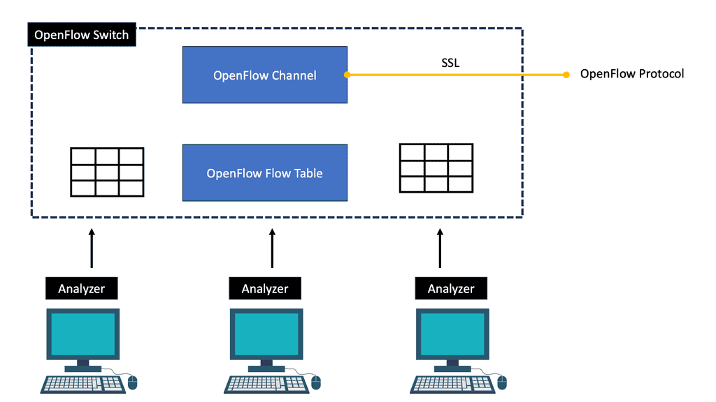
Building blocks: SDN Environment
As a fundamental building block of an SDN deployment, the controller, the SDN switch (for example, an OpenFlow switch), and the interfaces are present in the controller to communicate with forwarding devices, generally the southbound interface (OpenFlow) and the northbound interface (the network application interface).
In an SDN, switches function as basic forwarding hardware, accessible via an open interface, with the control logic and algorithms offloaded to controllers. Hybrid (OpenFlow-enabled) and pure (OpenFlow-only) OpenFlow switches are available.
OpenFlow switches rely entirely on a controller for forwarding decisions, without legacy features or onboard control. Hybrid switches support OpenFlow as well, in addition to traditional operation and protocols. Today, hybrid switches are the most common type of commercial switch. A flow table performs packet lookup and forwarding in an OpenFlow switch.
### The Role of the OpenFlow Controller
The OpenFlow controller is the brain of the SDN, orchestrating the flow of data across the network. It communicates with the network devices using the OpenFlow protocol to dictate how packets should be handled. The controller’s primary function is to make decisions on the path data packets should take, ensuring optimal network performance and resource utilization. This centralization of control allows for dynamic network configuration, paving the way for innovative applications and services.
### OpenFlow Switches: The Workhorses of the Network
While the controller is the brain, OpenFlow switches are the workhorses, executing the instructions they receive. These switches operate at the data plane, where they forward packets based on the rules set by the controller. Each switch maintains a flow table that matches incoming packets to particular actions, such as forwarding or dropping the packet. This separation of control and data planes is what sets SDN apart from traditional networking, offering unparalleled flexibility and control.
### Flow Tables: The Heart of OpenFlow Switches
Flow tables are the core component of OpenFlow switches, dictating how packets are handled. Each entry in a flow table consists of match fields, counters, and a set of instructions. Match fields identify the packets that should be affected by the rule, counters track the number of packets and bytes that match the entry, and instructions define the actions to be taken. This modular approach allows for precise traffic management and is essential for implementing advanced network policies.
OpenFlow Table & Routing Tables
### What is an OpenFlow Flow Table?
OpenFlow is a protocol that allows network controllers to interact with the forwarding plane of network devices like switches and routers. At the heart of OpenFlow is the flow table. This table contains a set of flow entries, each specifying actions to take on packets that match a particular pattern. Unlike traditional routing tables, which rely on predefined paths and protocols, OpenFlow flow tables provide flexibility and programmability, allowing dynamic changes in how packets are handled based on real-time network conditions.
### Understanding Routing Tables
Routing tables are a staple of traditional networking, used by routers to determine the best path for forwarding packets to their final destinations. These tables consist of a list of network destinations, with associated metrics that help in selecting the most efficient route. Routing protocols such as OSPF, BGP, and RIP are employed to maintain and update these tables, ensuring that data flows smoothly across the interconnected web of networks. While reliable, routing tables are less flexible compared to OpenFlow flow tables, as changes in network traffic patterns require updates to routing protocols and configurations.
Example of a Routing Table
### Key Differences Between OpenFlow Flow Table and Routing Table
The primary distinction between OpenFlow flow tables and routing tables lies in their approach to network management. OpenFlow flow tables are dynamic and programmable, allowing for real-time adjustments and fine-grained control over traffic flows. This makes them ideal for environments where network agility and customization are paramount. Conversely, routing tables offer a more static and predictable method of packet forwarding, which can be beneficial in stable networks where consistency and reliability are prioritized.
### Use Cases: When to Use Each
OpenFlow flow tables are particularly advantageous in software-defined networking (SDN) environments, where network administrators need to quickly adapt to changing conditions and optimize traffic flows. They are well-suited for data centers, virtualized networks, and scenarios requiring high levels of automation and scalability. On the other hand, traditional routing tables are best used in established networks with predictable traffic patterns, such as those found in enterprise or service provider settings, where reliability and stability are key.
You may find the following useful for pre-information:
What is OpenFlow?
OpenFlow was the first protocol of the Software-Defined Networking (SDN) trend and is the only protocol that allows the decoupling of a network device’s control plane from the data plane. In most straightforward terms, the control plane can be thought of as the brains of a network device. On the other hand, the data plane can be considered hardware or application-specific integrated circuits (ASICs) that perform packet forwarding.
Numerous devices also support running OpenFlow in a hybrid mode, meaning OpenFlow can be deployed on a given port, virtual local area network (VLAN), or even within a regular packet-forwarding pipeline such that if there is not a match in the OpenFlow table, then the existing forwarding tables (MAC, Routing, etc.) are used, making it more analogous to Policy Based Routing (PBR).

What is SDN?
Despite various modifications to the underlying architecture and devices (such as switches, routers, and firewalls), traditional network technologies have existed since the inception of networking. Using a similar approach, frames and packets have been forwarded and routed in a limited manner, resulting in low efficiency and high maintenance costs. Consequently, the architecture and operation of networks need to evolve, resulting in SDN.
By enabling network programmability, SDN promises to simplify network control and management and allow innovation in computer networking. Network engineers configure policies to respond to various network events and application scenarios. They can achieve the desired results by manually converting high-level policies into low-level configuration commands.
Often, minimal tools are available to accomplish these very complex tasks. Controlling network performance and tuning network management are challenging and error-prone tasks.
A modern network architecture consists of a control plane, a data plane, and a management plane; the control and data planes are merged into a machine called Inside the Box. To overcome these limitations, programmable networks have emerged.
How OpenFlow Works:
At the core of OpenFlow is the concept of a flow table, which resides in each OpenFlow-enabled switch. The flow table contains match-action rules defining how incoming packets should be processed and forwarded. The centralized controller determines these rules and communicates using the OpenFlow protocol with the switches.
When a packet arrives at an OpenFlow-enabled switch, it is first matched against the rules in the flow table. If a match is found, the corresponding action is executed, including forwarding the packet, dropping it, or sending it to the controller for further processing. This decoupling of the control and data planes allows for flexible and programmable network management.
What is OpenFlow SDN?
The main goal of SDN is to separate the control and data planes and transfer network intelligence and state to the control plane. These concepts have been exploited by technologies like Routing Control Platform (RCP), Secure Architecture for Network Enterprise (SANE), and, more recently, Ethane.
In addition, there is often a connection between SDN and OpenFlow. The Open Networking Foundation (ONF) is responsible for advancing SDN and standardizing OpenFlow, whose latest version is 1.5.0.
An SDN deployment starts with these building blocks.
For communication with forwarding devices, the controller has the SDN switch (for example, an OpenFlow switch), the SDN controller, and the interfaces. An SDN deployment is based on two basic building blocks: a southbound interface (OpenFlow) and a northbound interface (the network application interface).
As the control logic and algorithms are offloaded to a controller, switches in SDNs may be represented as basic forwarding hardware. Switches that support OpenFlow come in two varieties: pure (OpenFlow-only) and hybrid (OpenFlow-enabled).
Pure OpenFlow switches do not have legacy features or onboard control for forwarding decisions. A hybrid switch can operate with both traditional protocols and OpenFlow. Hybrid switches make up the majority of commercial switches available today. In an OpenFlow switch, a flow table performs packet lookup and forwarding.
OpenFlow reference switch
The OpenFlow protocol and interface allow OpenFlow switches to be accessed as essential forwarding elements. A flow-based SDN architecture like OpenFlow simplifies switching hardware. Still, it may require additional forwarding tables, buffer space, and statistical counters that are difficult to implement in traditional switches with integrated circuits tailored to specific applications.
There are two types of switches in an OpenFlow network: hybrids (which enable OpenFlow) and pores (which only support OpenFlow). OpenFlow is supported by hybrid switches and traditional protocols (L2/L3). OpenFlow switches rely entirely on a controller for forwarding decisions and do not have legacy features or onboard control.
Hybrid switches are the majority of the switches currently available on the market. This link must remain active and secure because OpenFlow switches are controlled over an open interface (through a TCP-based TLS session). OpenFlow is a messaging protocol that defines communication between OpenFlow switches and controllers, which can be viewed as an implementation of SDN-based controller-switch interactions.
Identify the Benefits of OpenFlow
Application-driven routing. Users can control the network paths. | The networks paths.A way to enhance link utilization. |
An open solution for VM mobility. No VLAN reliability. | A means to traffic engineer without MPLS. |
A solution to build very large Layer 2 networks. | A way to scale Firewalls and Load Balancers. |
A way to configure an entire network as a whole as opposed to individual entities. | A way to build your own encryption solution. Off-the-box encryption. |
A way to distribute policies from a central controller. | Customized flow forwarding. Based on a variety of bit patterns. |
A solution to get a global view of the network and its state. End-to-end visibility. | A solution to use commodity switches in the network. Massive cost savings. |
The following table lists the Software Networking ( SDN ) benefits and the problems encountered with existing control plane architecture:
Identify the benefits of OpenFlow and SDN | Problems with the existing approach |
Faster software deployment. | Large scale provisioning and orchestration. |
Programmable network elements. | Limited traffic engineering ( MPLS TE is cumbersome ) |
Faster provisioning. | Synchronized distribution policies. |
Centralized intelligence with centralized controllers. | Routing of large elephant flows. |
Decisions are based on end-to-end visibility. | Qos and load based forwarding models. |
Granular control of flows. | Ability to scale with VLANs. |
Decreases the dependence on network appliances like load balancers. |
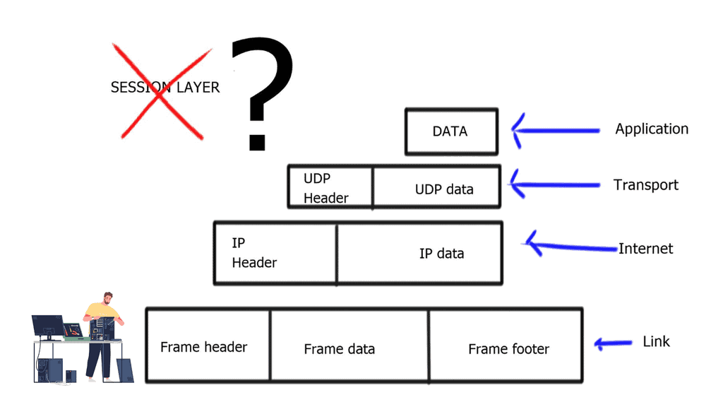
**A key point: The lack of a session layer in the TCP/IP stack**
Regardless of the hype and benefits of SDN, neither OpenFlow nor other SDN technologies address the real problems of the lack of a session layer in the TCP/IP protocol stack. The problem is that the client’s application ( Layer 7 ) connects to the server’s IP address ( Layer 3 ), and if you want to have persistent sessions, the server’s IP address must remain reachable.
This session’s persistence and the ability to connect to multiple Layer 3 addresses to reach the same device is the job of the OSI session layer. The session layer provides the services for opening, closing, and managing a session between end-user applications. In addition, it allows information from different sources to be correctly combined and synchronized.
The problem is the TCP/IP reference module does not consider a session layer, and there is none in the TCP/IP protocol stack. SDN does not solve this; it gives you different tools to implement today’s kludges.
Control and data plane
When we identify the benefits of OpenFlow, let us first examine traditional networking operations. Traditional networking devices have a control and forwarding plane, depicted in the diagram below. The control plane is responsible for setting up the necessary protocols and controls so the data plane can forward packets, resulting in end-to-end connectivity. These roles are shared on a single device, and the fast packet forwarding ( data path ) and the high-level routing decisions ( control path ) occur on the same device.
What is OpenFlow | SDN separates the data and control plane?
**Control plane**
The control plane is part of the router architecture and is responsible for drawing the network map in routing. When we mention control planes, you usually think about routing protocols, such as OSPF or BGP. But in reality, the control plane protocols perform numerous other functions, including:
Connectivity management ( BFD, CFM ) | Interface state management ( PPP, LACP ) |
Service provisioning ( RSVP for InServ or MPLS TE) | Topology and reachability information exchange ( IP routing protocols, IS-IS in TRILL/SPB ) |
Adjacent device discovery via HELLO mechanism | ICMP |
Control plane protocols run over data plane interfaces to ensure “shared fate” – if the packet forwarding fails, the control plane protocol fails as well.
Most control plane protocols ( BGP, OSPF, BFD ) are not data-driven. A BGP or BFD packet is never sent as a direct response to a data packet. There is a question mark over the validity of ICMP as a control plane protocol. The debate is whether it should be classed in the control or data plane category.
Some ICMP packets are sent as replies to other ICMP packets, and others are triggered by data plane packets, i.e., data-driven. My view is that ICMP is a control plane protocol that is triggered by data plane activity. After all, the “C” is ICMP does stand for “Control.”
**Data plane**
The data path is part of the routing architecture that decides what to do when a packet is received on its inbound interface. It is primarily focused on forwarding packets but also includes the following functions:
ACL logging | Netflow accounting |
NAT session creation | NAT table maintenance |
The data forwarding is usually performed in dedicated hardware, while the additional functions ( ACL logging, Netflow accounting ) typically happen on the device CPU, commonly known as “punting.” The data plane for an OpenFlow-enabled network can take a few forms.
However, the most common, even in the commercial offering, is the Open vSwitch, often called the OVS. The Open vSwitch is an open-source implementation of a distributed virtual multilayer switch. It enables a switching stack for virtualization environments while supporting multiple protocols and standards.
Software-defined networking changes the control and data plane architecture.
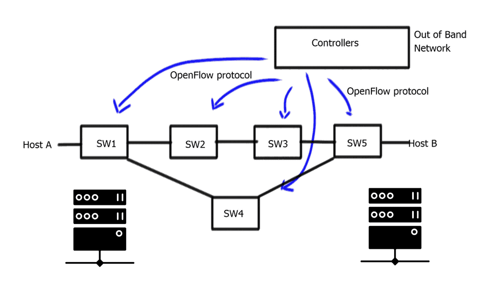
The concept of SDN separates these two planes, i.e., the control and forwarding planes are decoupled. This allows the networking devices in the forwarding path to focus solely on packet forwarding. An out-of-band network uses a separate controller ( orchestration system ) to set up the policies and controls. Hence, the forwarding plane has the correct information to forward packets efficiently.
In addition, it allows the network control plane to be moved to a centralized controller on a server instead of residing on the same box carrying out the forwarding. Moving the intelligence ( control plane ) of the data plane network devices to a controller enables companies to use low-cost, commodity hardware in the forwarding path. A significant benefit is that SDN separates the data and control plane, enabling new use cases.
A centralized computation and management plane makes more sense than a centralized control plane.
The controller maintains a view of the entire network and communicates with Openflow ( or, in some cases, BGP with BGP SDN ) with the different types of OpenFlow-enabled network boxes. The data path portion remains on the switch, such as the OVS bridge, while the high-level decisions are moved to a separate controller. The data path presents a clean flow table abstraction, and each flow table entry contains a set of packet fields to match, resulting in specific actions ( drop, redirect, send-out-port ).
When an OpenFlow switch receives a packet it has never seen before and doesn’t have a matching flow entry, it sends the packet to the controller for processing. The controller then decides what to do with the packet.
Applications could then be developed on top of this controller, performing security scrubbing, load balancing, traffic engineering, or customized packet forwarding. The centralized view of the network simplifies problems that were harder to overcome with traditional control plane protocols.
A single controller could potentially manage all OpenFlow-enabled switches. Instead of individually configuring each switch, the controller can push down policies to multiple switches simultaneously—a compelling example of many-to-one virtualization.
Now that SDN separates the data and control plane, the operator uses the centralized controller to choose the correct forwarding information per-flow basis. This allows better load balancing and traffic separation on the data plane. In addition, there is no need to enforce traffic separation based on VLANs, as the controller would have a set of policies and rules that would only allow traffic from one “VLAN” to be forwarded to other devices within that same “VLAN.”
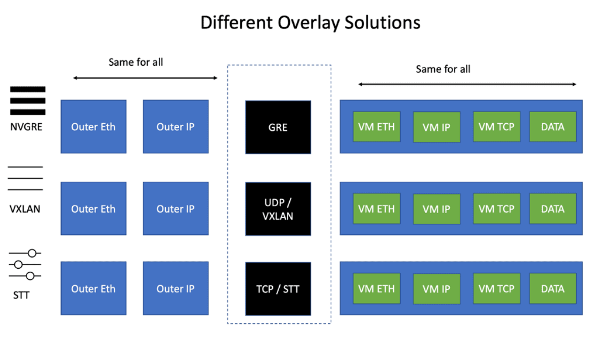
The advent of VXLAN
With the advent of VXLAN, which allows up to 16 million logical entities, the benefits of SDN should not be purely associated with overcoming VLAN scaling issues. VXLAN already does an excellent job with this. It does make sense to deploy a centralized control plane in smaller independent islands; in my view, it should be at the edge of the network for security and policy enforcement roles. Using Openflow on one or more remote devices is easy to implement and scale.
It also decreases the impact of controller failure. If a controller fails and its sole job is implementing packet filters when a new user connects to the network, the only affecting element is that the new user cannot connect. If the controller is responsible for core changes, you may have interesting results with a failure. New users not being able to connect is bad, but losing your entire fabric is not as bad.
A traditional networking device runs all the control and data plane functions. The control plane, usually implemented in the central CPU or the supervisor module, downloads the forwarding instructions into the data plane structures. Every vendor needs communications protocols to bind the two planes together to download forward instructions.
Therefore, all distributed architects need a protocol between control and data plane elements. The protocol binding this communication path for traditional vendor devices is not open-source, and every vendor uses its proprietary protocol (Cisco uses IPC—InterProcess Communication ).
Openflow tries to define a standard protocol between the control plane and the associated data plane. When you think of Openflow, you should relate it to the communication protocol between the traditional supervisors and the line cards. OpenFlow is just a low-level tool.
OpenFlow is a control plane ( controller ) to data plane ( OpenFlow enabled device ) protocol that allows the control plane to modify forwarding entries in the data plane. It enables SDN to separate the data and control planes.

Proactive versus reactive flow setup
OpenFlow operations have two types of flow setups: Proactive and Reactive.
With Proactive, the controller can populate the flow tables ahead of time, similar to a typical routing. However, the packet-in event never occurs by pre-defining your flows and actions ahead of time in the switch’s flow tables. The result is all packets are forwarded at line rate. With Reactive, the network devices react to traffic, consult the OpenFlow controller, and create a rule in the flow table based on the instruction. The problem with this approach is that there can be many CPU hits.
The following table outlines the critical points for each type of flow setup:
Proactive flow setup | Reactive flow setup |
Works well when the controller is emulating BGP or OSPF. | Used when no one can predict when and where a new MAC address will appear. |
The controller must first discover the entire topology. | Punts unknown packets to the controller. Many CPU hits. |
Discover endpoints ( MAC addresses, IP addresses, and IP subnets ) | Compute forwarding paths on demand. Not off the box computation. |
Compute off the box optimal forwarding. | Install flow entries based on actual traffic. |
Download flow entries to the data plane switches. | Has many scalability concerns such as packet punting rate. |
No data plane controller involvement with the exceptions of ARP and MAC learning. Line-rate performance. | Not a recommended setup. |
Hop-by-hop versus path-based forwarding
The following table illustrates the key points for the two types of forwarding methods used by OpenFlow: hop-by-hop forwarding and path-based forwarding:
Hop-by-hop Forwarding | Path-based Forwarding |
Similar to traditional IP Forwarding. | Similar to MPLS. |
Installs identical flows on each switch on the data path. | Map flows to paths on ingress switches and assigns user traffic to paths at the edge node |
Scalability concerns relating to flow updates after a change in topology. | Compute paths across the network and installs end-to-end path-forwarding entries. |
Significant overhead in large-scale networks. | Works better than hop-by-hop forwarding in large-scale networks. |
FIB update challenges. Convergence time. | Core switches don’t have to support the same granular functionality as edge switches. |
Obviously, with any controller, the controller is a lucrative target for attack. Anyone who knows you are using a controller-based network will try to attack the controller and its control plane. The attacker may attempt to intercept the controller-to-switch communication and replace it with its commands, essentially attacking the control plane with whatever means they like.
An attacker may also try to insert a malformed packet or some other type of unknown packet into the controller ( fuzzing attack ), exploiting bugs in the controller and causing the controller to crash.
Fuzzing attacks can be carried out with application scanning software such as Burp Suite. It attempts to manipulate data in a particular way, breaking the application.
The best way to tighten security is to encrypt switch-to-controller communications with SSL and self-signed certificates to authenticate the switch and controller. It would also be best to minimize interaction with the data plane, except for ARP and MAC learning.
To prevent denial-of-service attacks on the controller, you can use Control Plane Policing ( CoPP ) on Ingress to avoid overloading the switch and the controller. Currently, NEC is the only vendor implementing CoPP.
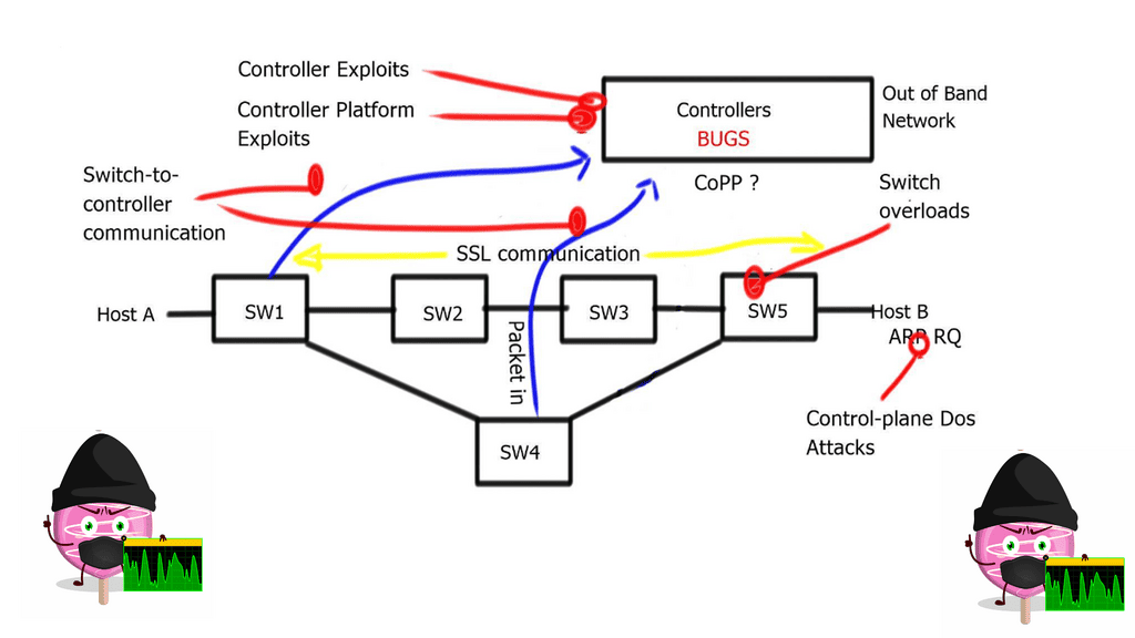
The Hybrid deployment model is helpful from a security perspective. For example, you can group specific ports or VLANs to OpenFlow and other ports or VLANs to traditional forwarding, then use traditional forwarding to communicate with the OpenFlow controller.
Software-defined networking or traditional routing protocols?
The move to a Software-Defined Networking architecture has clear advantages. It’s agile and can react quickly to business needs, such as new product development. For businesses to succeed, they must have software that continues evolving.
Otherwise, your customers and staff may lose interest in your product and service. The following table displays the advantages and disadvantages of the existing routing protocol control architecture.
+Reliable and well known. | -Non-standard Forwarding models. Destination-only and not load-aware metrics** |
+Proven with 20 plus years field experience. | -Loosely coupled. |
+Deterministic and predictable. | -Lacks end-to-end transactional consistency and visibility. |
+Self-Healing. Traffic can reroute around a failed node or link. | -Limited Topology discovery and extraction. Basic neighbor and topology tables. |
+Autonomous. | -Lacks the ability to change existing control plane protocol behavior. |
+Scalable. | -Lacks the ability to introduce new control plane protocols. |
+Plenty of learning and reading materials. |
** Basic EIGRP IETF originally proposed an Energy-Aware Control Plane, but the IETF later removed this.
Software-Defined Networking: Use Cases
Edge Security policy enforcement at the network edge. | Authenticate users or VMs and deploy per-user ACL before connecting a user to the network. |
Custom routing and online TE. | The ability to route on a variety of business metrics aka routing for dollars. Allowing you to override the default routing behavior. |
Custom traffic processing. | For analytics and encryption. |
Programmable SPAN ports | Use Openflow entries to mirror selected traffic to the SPAN port. |
DoS traffic blackholing & distributed DoS prevention. | Block DoS traffic as close to the source as possible with more selective traffic targeting than the original RTBH approach**. The traffic blocking is implemented in OpenFlow switches. Higher performance with significantly lower costs. |
Traffic redirection and service insertion. | Redirect a subset of traffic to network appliances and install redirection flow entries wherever needed. |
Network Monitoring. | The controller is the authoritative source of information on network topology and Forwarding paths. |
Scale-Out Load Balancing. | Punt new flows to the Openflow controller and install per-session entries throughout the network. |
IPS Scale-Out. | OpenFlow is used to distribute the load to multiple IDS appliances. |
**Remote-Triggered Black Hole: RTBH refers to installing a host route to a bogus IP address ( RTBH address ) pointing to NULL interfaces on all routers. BGP is used to advertise the host routes to other BGP peers of the attacked hosts, with the next hop pointing to the RTBH address, and it is mainly automated in ISP environments.
SDN deployment models
Guidelines:
- Start with small deployments away from the mission-critical production path, i.e., the Core. Ideally, start with device or service provisioning systems.
- Start at the Edge and slowly integrate with the Core. Minimize the risk and blast radius. Start with packet filters at the Edge and tasks that can be easily automated ( VLANs ).
- Integrate new technology with the existing network.
- Gradually increase scale and gain trust. Experience is key.
- Have the controller in a protected out-of-band network with SSL connectivity to the switches.
There are 4 different models for OpenFlow deployment, and the following sections list the key points of each model.
Native OpenFlow
- They are commonly used for Greenfield deployments.
- The controller performs all the intelligent functions.
- The forwarding plane switches have little intelligence and solely perform packet forwarding.
- The white box switches need IP connectivity to the controller for the OpenFlow control sessions. If you are forced to use an in-band network for this communication path using an isolated VLAN with STP, you should use an out-of-band network.
- Fast convergence techniques such as BFD may be challenging to use with a central controller.
- Many people believe that this approach does not work for a regular company. Companies implementing native OpenFlow, such as Google, have the time and resources to reinvent the wheel when implementing a new control-plane protocol ( OpenFlow ).
Native OpenFlow with Extensions
- Some control plane functions are handled from the centralized controller to the forwarding plane switches. For example, the OpenFlow-enabled switches could load balancing across multiple links without the controller’s previous decision. You could also run STP, LACP, or ARP locally on the switch without interaction with the controller. This approach is helpful if you lose connectivity to the controller. If the low-level switches perform certain controller functions, packet forwarding will continue in the event of failure.
- The local switches should support the specific OpenFlow extensions that let them perform functions on the controller’s behalf.
Hybrid ( Ships in the night )
- This approach is used where OpenFlow runs in parallel with the production network.
- The same network box is controlled by existing on-box and off-box control planes ( OpenFlow).
- Suitable for pilot deployment models as switches still run traditional control plane protocols.
- The Openflow controller manages only specific VLANs or ports on the network.
- The big challenge is determining and investigating the conflict-free sharing of forwarding plane resources across multiple control planes.
Integrated OpenFlow
- OpenFlow classifiers and forwarding entries are integrated with the existing control plane. For example, Juniper’s OpenFlow model follows this mode of operation where OpenFlow static routes can be redistributed into the other routing protocols.
- No need for a new control plane.
- No need to replace all forwarding hardware
- It is the most practical approach as long as the vendor supports it.
Closing Points on OpenFlow
OpenFlow is a communication protocol that provides access to the forwarding plane of a network switch or router over the network. It was initially developed at Stanford University and has since been embraced by the Open Networking Foundation (ONF) as a core component of SDN. OpenFlow allows network administrators to program the control plane, enabling them to direct how packets are forwarded through the network. This decoupling of the control and data planes is what empowers SDN to offer more dynamic and flexible network management.
The architecture of OpenFlow is quite straightforward yet powerful. It consists of three main components: the controller, the switch, and the protocol itself. The controller is the brains of the operation, managing network traffic by sending instructions to OpenFlow-enabled switches. These switches, in turn, execute the instructions received, altering the flow of network data accordingly. This setup allows for centralized network control, offering unprecedented levels of automation and agility.
**Advantages of OpenFlow**
OpenFlow brings several critical advantages to network management and control:
1. Flexibility and Programmability: With OpenFlow, network administrators can dynamically reconfigure the behavior of network devices, allowing for greater adaptability to changing network requirements.
2. Centralized Control: By centralizing control in a single controller, network administrators gain a holistic view of the network, simplifying management and troubleshooting processes.
3. Innovation and Experimentation: OpenFlow enables researchers and developers to experiment with new network protocols and applications, fostering innovation in the networking industry.
4. Scalability: OpenFlow’s centralized control architecture provides the scalability needed to manage large-scale networks efficiently.
**Implications for Network Control**
OpenFlow has significant implications for network control, paving the way for new possibilities in network management:
1. Software-Defined Networking (SDN): OpenFlow is a critical component of the broader concept of SDN, which aims to decouple network control from the underlying hardware, providing a more flexible and programmable infrastructure.
2. Network Virtualization: OpenFlow facilitates network virtualization, allowing multiple virtual networks to coexist on a single physical infrastructure.
3. Traffic Engineering: By controlling the flow of packets at a granular level, OpenFlow enables advanced traffic engineering techniques, optimizing network performance and resource utilization.
OpenFlow represents a paradigm shift in network control, offering a more flexible, scalable, and programmable approach to managing networks. By separating the control and data planes, OpenFlow empowers network administrators to have fine-grained control over network behavior, improving efficiency, innovation, and adaptability. As the networking industry continues to evolve, OpenFlow and its related technologies will undoubtedly play a crucial role in shaping the future of network management.
What is VXLAN
Understanding VXLAN Basics
It is essential to grasp VXLAN’s fundamental concepts to comprehend it. VXLAN enables the creation of virtualized Layer 2 networks over an existing Layer 3 infrastructure. It uses encapsulation techniques to extend Layer 2 segments over long distances, enabling flexible deployment of virtual machines across physical hosts and data centers.
VXLAN Encapsulation: One of the key components of VXLAN is encapsulation. When a virtual machine sends data across the network, VXLAN encapsulates the original Ethernet frame within a new UDP/IP packet. This encapsulated packet is then transmitted over the underlying Layer 3 network, allowing for seamless communication between virtual machines regardless of their physical location.
VXLAN Tunneling: VXLAN employs tunneling to transport the encapsulated packets between VXLAN-enabled devices. These devices, known as VXLAN Tunnel Endpoints (VTEPs), establish tunnels to carry VXLAN traffic. By leveraging tunneling protocols like Generic Routing Encapsulation (GRE) or Virtual Extensible LAN (VXLAN-GPE), VTEPs ensure the delivery of encapsulated packets across the network.
**Benefits of VXLAN**
VXLAN brings numerous benefits to modern network architectures. It enables network virtualization and multi-tenancy, allowing for the efficient and secure isolation of network segments. VXLAN also provides scalability, as it can support a significantly higher number of virtual networks than traditional VLAN-based networks. Additionally, VXLAN facilitates workload mobility and disaster recovery, making it an ideal choice for cloud environments.
**Implementing VXLAN**
VXLAN Implementation Considerations: While VXLAN offers immense advantages, there are a few considerations to consider when implementing it. VXLAN requires network devices that support the technology, including VTEPs and VXLAN-aware switches. It is also crucial to properly configure and manage the VXLAN overlay network to ensure optimal performance and security.
Data centers evolution
In recent years, data centers have seen a significant evolution. This evolution has brought popular technologies such as virtualization, cloud computing (private, public, and hybrid), and software-defined networking (SDN). Mobile-first and cloud-native data centers must scale, be agile, secure, consolidate, and integrate with compute/storage orchestrators. As well as visibility, automation, ease of management, operability, troubleshooting, and advanced analytics, today’s data center solutions are expected to include many other features.
A more service-centric approach is replacing device-by-device management. Most requests for proposals (RFPs) specify open application programming interfaces (APIs) and standards-based protocols to prevent vendor lock-in. A Cisco Virtual Extensible LAN (VXLAN)-based fabric using Nexus switches2 and NX-OS controllers form Cisco Virtual Extensible LAN (VXLAN).
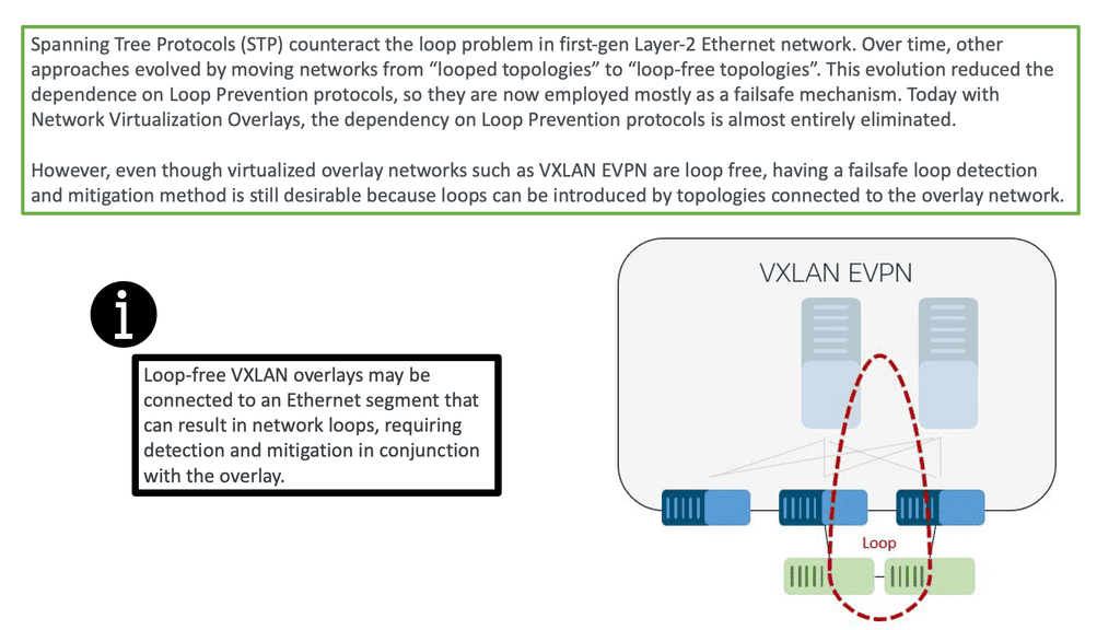
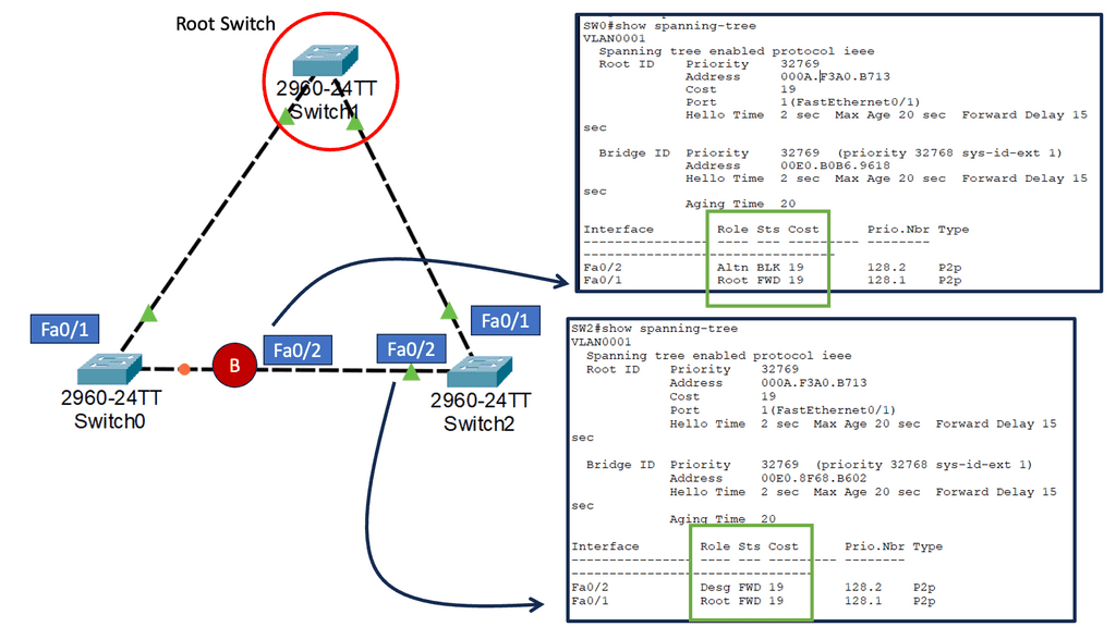
Issues with STP
When a switch receives redundant paths, the spanning tree protocol must designate one of those paths as blocked to prevent loops. While this mechanism is necessary, it can lead to suboptimal network performance. Blocked ports limit bandwidth utilization, which can be particularly problematic in environments with heavy data traffic.
One significant concern with the spanning tree protocol is its slow convergence time. When a network topology changes, the protocol takes time to recompute the spanning tree and reestablish connectivity. During this convergence period, network downtime can occur, disrupting critical operations and causing frustration for users.
What is VXLAN?
The Internet Engineering Task Force (IETF) developed VXLAN, or Virtual eXtensible Local-Area Network, as a network virtualization technology standard. Multi-tenant networks allow multiple organizations to share a physical network without accessing each other’s traffic.
The VXLAN can be compared to individual apartment apartments: each apartment is a separate, private dwelling within a shared physical structure, just as each VXLAN is a discrete, private network segment within a shared physical infrastructure.
With VXLANs, physical networks can be segmented into 16 million logical networks. To encapsulate Layer 2 Ethernet frames, User Datagram Protocol (UDP) packets with a VXLAN header are used. Combining VXLAN with Ethernet virtual private networks (EVPNs), which transport Ethernet traffic over WAN protocols, allows Layer 2 networks to be extended across Layer 3 IP or MPLS networks.
**Benefits of VXLAN:**
– Scalability: VXLAN allows creating up to 16 million logical networks, providing the scalability required for large-scale virtualized environments.
– Network Segmentation: By leveraging VXLAN, organizations can segment their networks into virtual segments, enhancing security and isolating traffic between applications or user groups.
– Flexibility and Mobility: VXLAN enables the movement of VMs across physical servers and data centers without the need to reconfigure network settings. This flexibility is crucial for workload mobility in dynamic environments.
– Interoperability: VXLAN is an industry-standard protocol supported by various networking vendors, ensuring compatibility across different network devices and platforms.
**Use Cases for VXLAN**
– Data Center Interconnect (DCI): VXLAN allows organizations to interconnect multiple data centers, enabling seamless workload migration, disaster recovery, and workload balancing across different locations.
– Multi-Tenant Environments: VXLAN enables service providers to offer virtualized network services to multiple tenants securely and isolatedly. This is particularly useful in cloud computing environments.
– Network Virtualization: VXLAN plays a crucial role in network virtualization, allowing organizations to create virtual networks independent of the underlying physical infrastructure. This enables greater flexibility and agility in managing network resources.
**VXLAN vs. GRE**
VXLAN, an overlay network technology, is designed to address the limitations of traditional VLANs. It enables the creation of virtual networks over an existing Layer 3 infrastructure, allowing for more flexible and scalable network deployments. VXLAN operates by encapsulating Layer 2 Ethernet frames within UDP packets, extending Layer 2 domains across Layer 3 boundaries.
GRE, on the other hand, is a simple IP packet encapsulation protocol. It provides a mechanism for encapsulating arbitrary protocols over an IP network and is widely used for creating point-to-point tunnels. GRE encapsulates the payload packets within IP packets, making it a versatile option for connecting remote networks securely.
Point-to-point GRE networks serve as a foundational element in modern networking. They allow for encapsulation and efficient transmission of various protocols over an IP network. Point-to-point GRE networks enable seamless communication and data transfer by establishing a direct virtual link between two endpoints.
Understanding mGRE
mGRE serves as the foundation for building DMVPN networks. It allows multiple sites to communicate with each other over a shared public network infrastructure while maintaining security and scalability. By utilizing a single mGRE tunnel interface on a central hub router, multiple spoke routers can dynamically establish and tear down tunnels, enabling seamless communication across the network.
The utilization of mGRE within DMVPN offers several key advantages. First, it simplifies network configuration by eliminating the need for point-to-point tunnels between each spoke router. Second, mGRE provides scalability, allowing for the dynamic addition or removal of spoke routers without impacting the overall network infrastructure. Third, mGRE enhances network resiliency by supporting multiple paths and providing load-balancing mechanisms.
Key VXLAN advantages
Because VXLANs are encapsulated inside UDP packets, they can run on any network that can send UDP packets. No matter how physically or geographically far a VTEP is from the decapsulating VTEP, it must forward UDP datagrams.
VXLAN and EVPN enable operators to create virtual networks from physical ports on any Layer 3 network switch supporting the standard. Connecting a port on switch A to two ports on switch B and another port on switch C creates a virtual network that appears to all connected devices as one physical network. Devices in this virtual network cannot see VXLANs or the underlying network fabric.
**Problems that VXLAN solves**
In the same way, as server virtualization has increased agility and flexibility, decoupling virtual networks from physical infrastructure has done the same. Therefore, network operators can scale their infrastructure rapidly and economically to meet growing demand while securely sharing a single physical network. For privacy and security reasons, networks are segmented to prevent one tenant from seeing or accessing the traffic of another.
In a similar way to traditional virtual LANs (VLANs), VXLANs enable operators to overcome the scaling limitations associated with VLANs.
- Up to 16 million VXLANs can be created in an administrative domain, compared to 4094 traditional VLANs. Cloud and service providers can segment networks using VXLANs to support many tenants.
- By using a VXLAN, you can create network segments between different data centers. In traditional VLAN networks, broadcast domains are created by segmenting traffic by VLAN tags, but once a packet containing VLAN tags reaches a router, the VLAN information is removed. There is no limit to the distance VLANs can travel within a Layer 2 network. Layer 3 boundaries, such as virtual machine migration, are generally avoided in certain use cases. Segmenting networks based on VXLAN encapsulates packets as UDP packets, while segmenting networks based on VXLAN encapsulates packets as IP packets. A virtual overlay network can extend as far as the physical Layer 3 routed network can reach when all switches and routers in the path support VXLAN without the applications running on the overlay network having to cross any Layer 3 boundaries. Servers connected to the network are still part of the Layer 2 network, even though UDP packets may have transited one or more routers.
- Using Layer 2 segmentation on top of an underlying Layer 3 network allows one to segment a Layer 2 network over an underlying Layer 3 network and support many network segments. By providing Layer 2 segmentation on top of an underlying Layer 3 network, Layer 2 networks can remain small even if they are distant. Smaller Layer 2 networks can prevent MAC table overflows on switches.
Primary VXLAN applications
A service provider or cloud provider deploys VXLAN for apparent reasons: they have many tenants or customers, and they must separate the traffic of one customer from another due to legal, privacy, and ethical considerations.
Users, departments, or other groups of network-segmented devices may be tenants in enterprise environments for security reasons. Isolating IoT network traffic from production network applications is a good security practice for Internet of Things (IoT) devices such as data center environmental sensors.
VXLAN has been widely adopted and is now used in many large enterprise networks for virtualization and cloud computing. It provides:
- A secure and efficient way to create virtual networks.
- Allowing for the creation of multi-tenant segmentation.
- Efficient routing.
- Hardware-agnostic capabilities.
With its widespread adoption, VXLAN has become an essential technology for network virtualization.
Example: VXLAN Flood and Learn
Understanding VXLAN Flood and Learn
VXLAN flood and learn handles unknown unicast, multicast, and broadcast traffic in VXLAN networks. It allows the network to learn and forward traffic to the appropriate destination without relying on traditional flooding techniques. By leveraging multicast, VXLAN flood and learn improves efficiency and reduces the network’s reliance on flooding every unknown packet.
Proper multicast group management is essential to implementing VXLAN flood and learning with multicast. VXLAN uses multicast groups to distribute unknown traffic efficiently within the network.
VXLAN flood and learn with multicast offers several benefits for data center networks. Firstly, it reduces the flooding of unknown traffic, which helps minimize network congestion and improves overall performance. Additionally, it allows for better scalability by avoiding the need to flood every unknown packet to all VTEPs (VXLAN Tunnel Endpoint). This results in more efficient network utilization and reduced processing overhead.
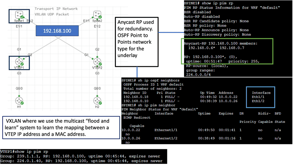

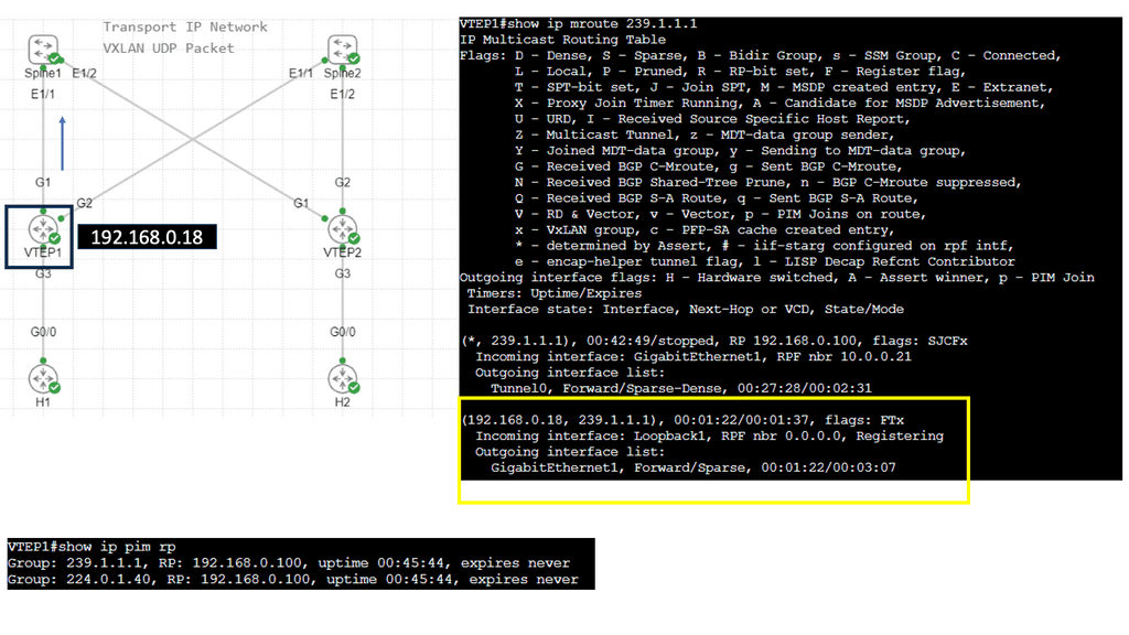
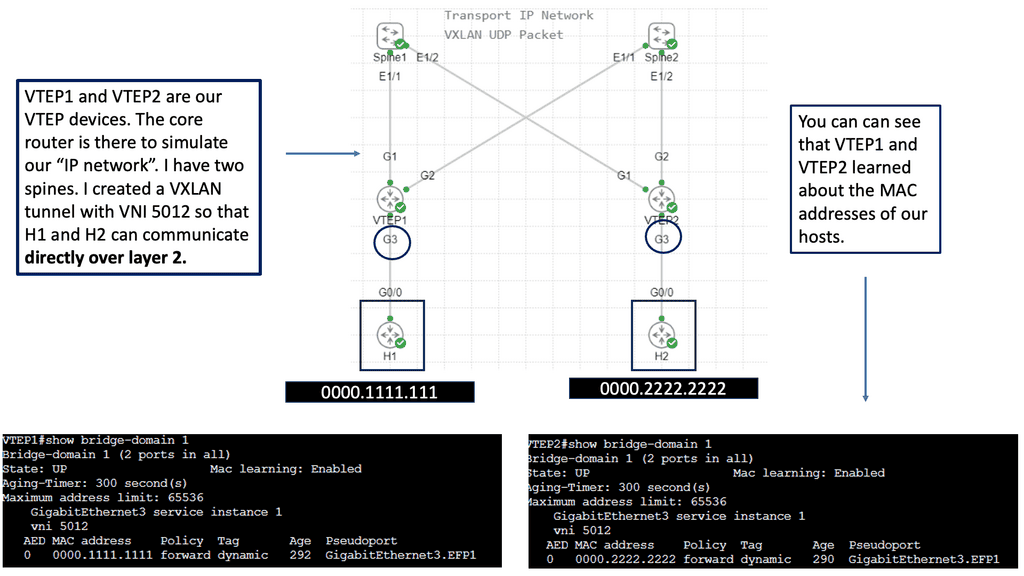
Related: Before you proceed, you may find the following posts helpful for pre-information:
Traditional layer two networks have issues because of the following reasons:
- Spanning tree: Restricts links.
- Limited amount of VLANs: Restricts scalability;
- Large MAC address tables: Restricts scalability and mobility
Spanning-tree avoids loops by blocking redundant links. By blocking connections, we create a loop-free topology and pay for links we can’t use. Although we could switch to a layer three network, some technologies require layer two networking.
VLAN IDs are 12 bits long, so we can create 4094 VLANs (0 and 4095 are reserved). Data centers may need help with only 4094 available VLANs. Let’s say we have a service provider with 500 customers. There are 4094 available VLANs, so each customer can only have eight.
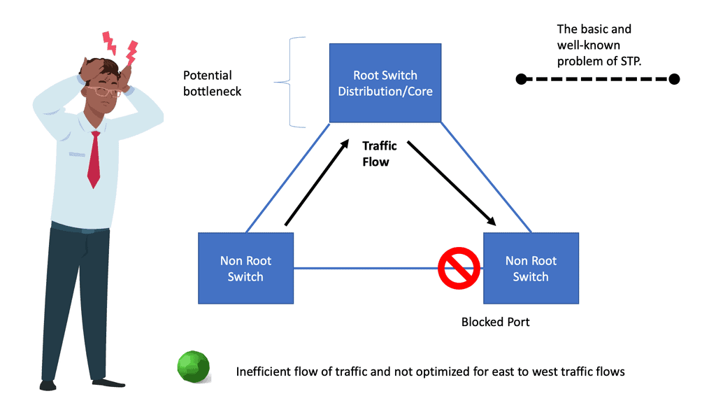
The Role of Server Virtualization
Server virtualization has exponentially increased the number of addresses in our switches’ MAC addresses. Before server virtualization, there was only one MAC address per switch port. With server virtualization, we can run many virtual machines (VMs) or containers on a single physical server. Virtual NICs and virtual MAC addresses are assigned to each virtual machine. One switch port must learn many MAC addresses.
A data center could connect 24 or 48 physical servers to a top-of-rack (ToR) switch. Since there may be many racks in a data center, each switch must store the MAC addresses of all VMs that communicate. Networks without server virtualization require much larger MAC address tables.
Guide: VXLAN
In the following lab, I created a Layer 2 overlay with VXLAN over a Layer 3 core. A bridge domain VNI of 6001 must match both sides of the overlay tunnel. What Is a VNI? The VLAN ID field in an Ethernet frame has only 12 bits, so VLAN cannot meet isolation requirements on data center networks. The emergence of VNI specifically solves this problem.
Note: The VNI
A VNI is a user identifier similar to a VLAN ID. A VNI identifies a tenant. VMs with different VNIs cannot communicate at Layer 2. During VXLAN packet encapsulation, a 24-bit VNI is added to a VXLAN packet, enabling VXLAN to isolate many tenants.
In the screenshot below, you will notice that I can ping from desktop 0 to desktop one even though the IP addresses are not in the routing table of the core devices, simulating a Layer 2 overlay. Consider VXLAN to be the overlay and the routing Layer 3 core to be the underlay.
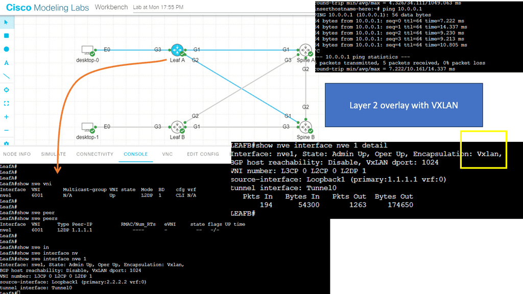
In the following screenshot, notice that the VNI has been changed. The VNI needs to be changed in two places in the configuration, as illustrated below. Once changed, the Peers are down; however, the NVE interface remains up. The VXLAN layer two overlay is not operational.
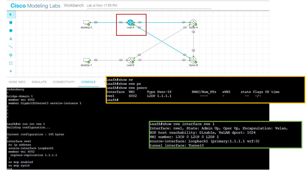
How does VXLAN work?
VXLAN uses tunneling to encapsulate Layer 2 Ethernet frames within IP packets. Each VXLAN network is identified by a unique 24-bit segment ID, the VXLAN Network Identifier (VNI). The source VM encapsulates the original Ethernet frame with a VXLAN header, including the VNI. The encapsulated packet is then sent over the physical IP network to the destination VM and decapsulated to retrieve the original Ethernet frame.
Analysis:
Notice below that it is running a ping from desktop 0 to desktop 1. The IP addresses assigned to this host are 10.0.0.1 and 10.0.0.2. First, notice that the ping is booming. When I do a packet capture on the links Gi1 connected to Leaf A, we see the encapsulation of the ICMP echo request and reply.
Everything is encapsulated into UDP port 1024. In my configurations of Leaf A and Leaf B, I explicitly set the VXLAN port to 1024.
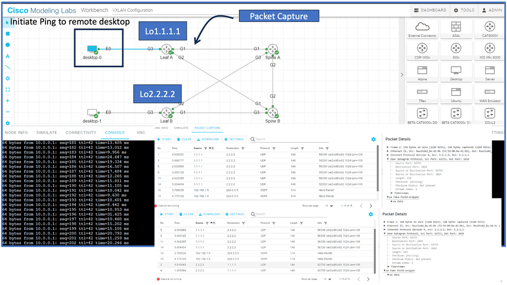
XLAN and Network Virtualization.
VXLAN and network virtualization
VXLAN is a form of network virtualization. Network virtualization cuts a single physical network into many virtual networks, often called network overlays. Virtualizing a resource allows it to be shared by multiple users. Virtualization provides the illusion that each user is on his or her resources.
In the case of virtual networks, each user is under the misconception that there are no other users of the network. To preserve the illusion, virtual networks are separated from one another. Packets cannot leak from one virtual network to another.
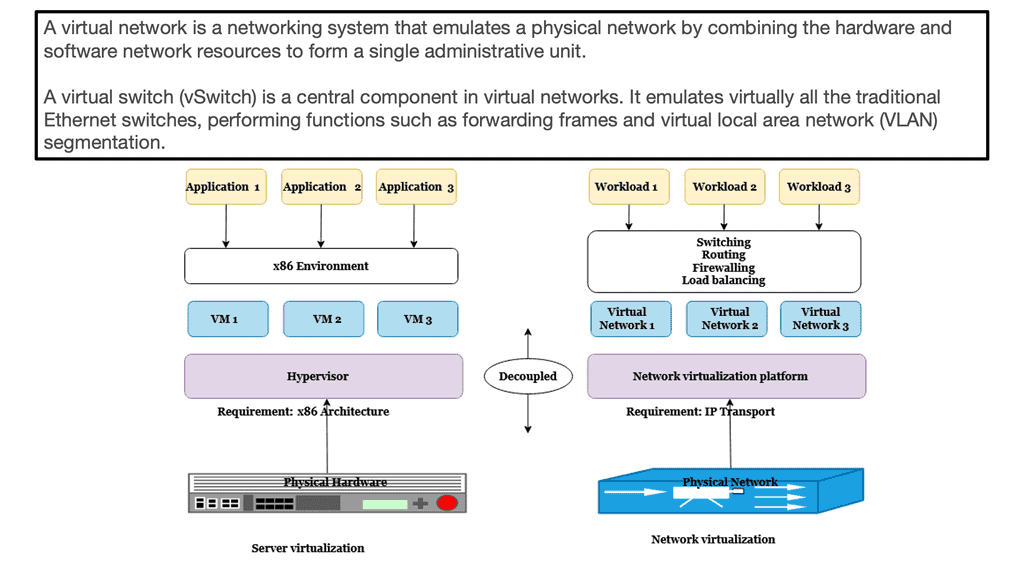
VXLAN Loop Detection and Prevention
So, before we dive into the benefits of VXLAN, let us address the basics of loop detection and prevention, which is a significant driver for using network overlays such as VLXAN. The challenge is that data frames can exist indefinitely when loops occur, disrupting network stability and degrading performance.
In addition, loops introduce broadcast radiation, increasing CPU and network bandwidth utilization, which degrades user application access experience. Finally, in multi-site networks, a loop can span multiple data centers, causing disruptions that are difficult to pinpoint. Overlay networking can solve much of this.
VXLAN vs VLAN
However, first-generation Layer-2 Ethernet networks could not natively detect or mitigate looped topologies, while modern Layer-2 overlays implicitly build loop-free topologies. Therefore, overlays do not need loop detection and mitigation as long as no first-gen Layer-2 network is attached. Essentially, there is no need for a VXLAN spanning tree.
So, one of the differences between VXLAN vs VLAN is that the VLAN has a 12-bit VID while VXLAN has a 24-bit VID network identifier, allowing you to create up to 16 million segments. VXLAN has tremendous scale and stable loop-free networking and is a foundation technology in the ACI Cisco.
VXLAN and Data Center Interconnect
VXLAN has revolutionized data center interconnect by providing a scalable, flexible, and efficient solution for extending Layer 2 networks. Its ability to enable network segmentation, multi-tenancy support, and seamless mobility makes it a valuable technology for modern businesses.
However, careful planning, consideration of network infrastructure, and security measures are essential for successful implementation. By harnessing the power of VXLAN, organizations can achieve a more agile, scalable, and interconnected data center environment.
VXLAN vs VLAN: The VXLAN Benefits Drive Adoption
Introduced by Cisco and VMware and now heavily used in open networking, VXLAN stands for Virtual eXtensible Local Area Network. It is perhaps the most popular overlay technology for IP-based SDN data centers and is used extensively with ACI networks.
VXLAN was explicitly designed for Layer 2 over Layer 3 tunneling. Its early competition from NVGRE and STT is fading away, and VXLAN is becoming the industry standard. VLXAN brings many advantages, especially in loop prevention, as there is no need for a VXLAN spanning tree.
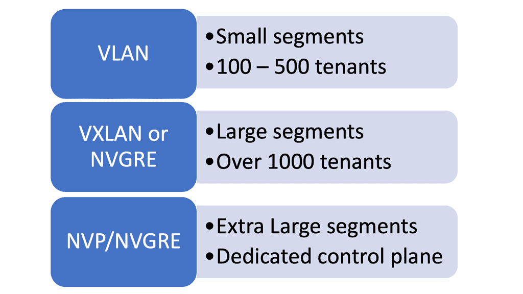
Today, overlays such as VXLAN almost eliminate the dependency on loop prevention protocols. However, even though virtualized overlay networks such as VXLAN are loop-free, having a failsafe loop detection and mitigation method is still desirable because loops can be introduced by topologies connected to the overlay network.
Loop prevention traditionally started with Spanning Tree Protocols (STP) to counteract the loop problem in first-gen Layer-2 Ethernet networks. Over time, other approaches evolved by moving networks from “looped topologies” to “loop-free topologies.
While LAG and MLAG were used, other approaches for building loop-free topologies arose using ECMP at the MAC or IP layers. For example, FabricPath or TRILL is a MAC layer ECMP approach that emerged in the last decade. More recently, network virtualization overlays that build loop-free topologies on top of IP layer ECMP became state-of-the-art.
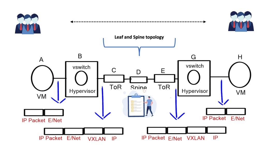
VXLAN vs VLAN: Why Introduce VXLAN?
- STP issues and scalability constraints: STP is undesirable on a large scale and lacks a proper load-balancing mechanism. A solution was needed to leverage the ECMP capabilities of an IP network while offering extended VLANs across an IP core, i.e., virtual segments across the network core. There is no VXLAN spanning tree.
- Multi-tenancy: Layer 2 networks are capped at 4000 VLANs, restricting multi-tenancy design—a big difference in the VXLAN vs VLAN debates.
- ToR table scalability: Every ToR switch may need to support several virtual servers, and each virtual server requires several NICs and MAC addresses. This pushes the limits on the ToR switch’s table sizes. In addition, after the ToR tables become full, Layer 2 traffic will be treated as unknown unicast traffic, which will be flooded across the network, causing instability to a previously stable core.
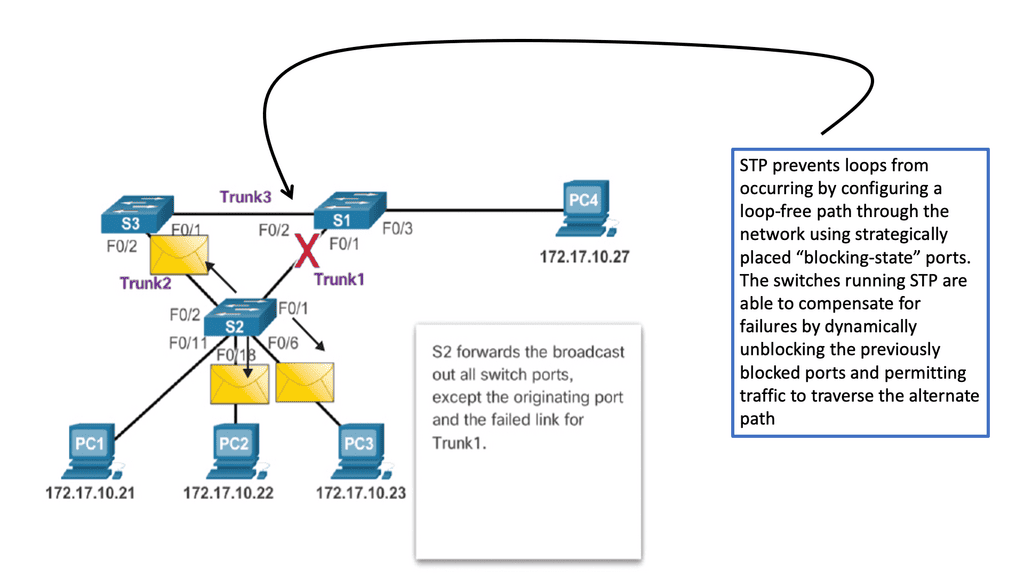
VXLAN use cases
Use Case | VXLAN Details |
Use Case 1 | Multi-tenant IaaS Clouds where you need a large number of segments |
Use Case 2 | Link Virtual to Physical Servers. This is done via software or hardware VXLAN to VLAN gateway |
Use Case 3 | HA Clusters across failure domains/availability zones |
Use Case 4 | VXLAN works well over fabrics that have equidistant endpoints |
Use Case 5 | VXLAN-encapsulated VLAN traffic across availability zones must be rate-limited to prevent broadcast storm propagation across multiple availability zones |
What is VXLAN? The operations
When discussing VXLAN vs VLAN, VXLAN employs a MAC over IP/UDP overlay scheme and extends the traditional VLAN boundary of 4000 VLANs. The 12-bit VLAN identifier in traditional VLANs capped scalability within the SDN data center and proved cumbersome if you wanted a VLAN per application segment model. VXLAN scales the 12-bit to a 24-bit identifier and allows for 16 million logical endpoints, with each endpoint potentially offering another 4,000 VLANs.
While tunneling does provide Layer 2 adjacency between these logical endpoints and allows VMs to move across boundaries, the main driver for its insertion was to overcome the challenge of having only 4000 VLAN.
Typically, an application segment has multiple segments; between each segment, you will have firewalling and load-balancing services, and each segment requires a different VLAN. The Layer 2 VLAN segment transfers non-routable heartbeats or state information that can’t cross an L3 boundary. You will soon reach the 4000k VLAN limit if you are a cloud provider.
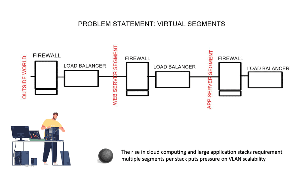
The control plane
The control plane is very similar to the spanning tree control plane. If a switch receives a packet destined for an unknown address, the switch will forward the packet to an IP address that floods the packet to all the other switches.
This IP address is, in turn, mapped to a multicast group across the network. VXLAN doesn’t explicitly have a control plane and requires an IP multicast running in the core for forwarding traffic and host discovery.
**Best practices for enabling IP Multicast in the core**
IP Multicast | In the Core |
The requirement for IP multicast in the core made VXLAN undesirable from an operation point of view. For example, creating the tunnel endpoints is simple, but introducing a protocol like IP multicast to a core just for the tunnel control plane was considered undesirable. As a result, some of the more recent versions of VXLAN support IP unicast.
VXLAN uses a MAC over IP/UDP solution to eliminate the need for a spanning tree. There is no VXLAN spanning tree. This enables the core to be IP and not run a spanning tree. Many people ask why VXLAN uses UDP. The reason is that the UDP port numbers cause VXLAN to inherit Layer 3 ECMP features. The entropy that enables load balancing across multiple paths is embedded into the UDP source port of the overlay header.
2nd Lab Guide: Multicast VLXAN
In this lab guide, we will look at a VXLAN multicast mode. The multicat mode requires both unicast and multicast connectivity between sites. Similar to the previous one, this configuration guide uses OSPF to provide unicast connectivity, and now we have an additional bidirectional Protocol Independent Multicast (PIM) to provide multicast connectivity.
This does not mean that you don’t have a multicast-enabled core. It would be best if you still had multicast enabled on the core.
So we are not tunneling multicast over an IPv4 core without having multicast enabled on the core. I have multicast on all Layer 3 interfaces, and the mroute table is populated on all Layer 3 routers. With the command: Show ip mroute, we are tunneling the multicast traffic, and with the command: Show nve vni, we have multicast group 239.0.0.10 and a state of UP.
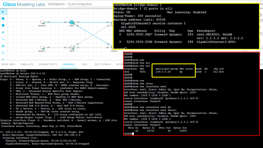
VXLAN benefits and stability
The underlying control plan network impacts the stability of VXLAN and the applications running within it. For example, if the underlying IP network cannot converge quickly enough, VLXAN packets may be dropped, and an application cache timeout may be triggered.
The rate of change in the underlying network significantly impacts the stability of the tunnels, yet the rate and change of the tunnels do not affect the underlying control plane. This is similar to how the strength of an MPLS / VPN overlay is affected by the core’s IGP.
VXLAN Points | VXLAN benefits | VXLAN drawbacks |
Point 1 | Runs over IP Transport | No control plane |
Point 2 | Offers a large number of logical endpoints | Needs IP Multicast*** |
Point 3 | Reduced flooding scope | No IGMP snooping ( yet ) |
Point 4 | Eliminates STP | No Pvlan support |
Point 5 | Easily integrated over existing Core | Requires Jumbo frames in the core ( 50 bytes) |
Point 6 | Minimal host-to-network integration | No built-in security features ** |
Point 7 | Not a DCI solution ( no arp reduction, first-hop gateway localization, no inbound traffic steering i.e, LISP ) |
** VXLAN has no built-in security features. Anyone who gains access to the core network can insert traffic into segments. The VXLAN transport network must be secure, as no existing firewall or intrusion prevention system (IPS) equipment can be seen in the VXLAN traffic.
*** Recent versions have Unicast VXLAN. Nexus 1000V release 4.2(1)SV2(2.1)
Updated: VXLAN enhancements
MAC distribution mode is an enhancement to VXLAN that prevents unknown unicast flooding and eliminates data plane MAC address learning. Traditionally, this was done by flooding to locate an unknown end host, but it has now been replaced with a control plane solution.
During VM startup, the VSM ( control plane ) collects the list of MAC addresses and distributes the MAC-to-VTEP mappings to all VEMs participating in a VXLAN segment. This technique makes VXLAN more optimal by unicasting more intelligently, similar to Nicira and VMware NVP.
ARP termination works by giving the VSM controller all the ARP and MAC information. This enables the VSM to proxy and respond locally to ARP requests without sending a broadcast. Because 90% of broadcast traffic is ARP requests ( ARP reply is unicast ), this significantly reduces broadcast traffic on the network.
Closing Points on VXLAN
VXLAN is a network virtualization technology that encapsulates Ethernet frames within UDP packets, allowing the creation of a virtual network overlay. This overlay extends beyond traditional VLANs, providing more address space and enabling communication across different physical networks. With a 24-bit segment ID, VXLAN supports up to 16 million unique network segments, compared to the 4096 segments possible with VLANs.
At its core, VXLAN uses tunneling to encapsulate Layer 2 frames within Layer 3 packets. This process involves two key components: the VXLAN Tunnel Endpoint (VTEP) and the VXLAN header. VTEPs are responsible for encapsulating and decapsulating the Ethernet frames. They also handle the communication between different network segments, ensuring seamless data transmission across the network.
The adoption of VXLAN brings several advantages to network management:
1. **Scalability**: VXLAN’s ability to support millions of network segments allows for unprecedented scalability, making it ideal for large-scale data centers.
2. **Flexibility**: By decoupling the network overlay from the physical infrastructure, VXLAN enables flexible network designs that can adapt to changing business needs.
3. **Improved Resource Utilization**: VXLAN optimizes the use of network resources, enhancing performance and reducing congestion by spreading traffic across multiple paths.
VXLAN is particularly beneficial in scenarios where network scalability and flexibility are paramount. Common use cases include:
– **Data Center Interconnect**: Connecting multiple data centers over a single, unified network fabric.
– **Multi-Tenant Environments**: Providing isolated network segments for different tenants in cloud environments.
– **Disaster Recovery**: Facilitating seamless failover and recovery by extending network segments across geographically dispersed locations.

Routing Convergence
Understanding Convergence
Router convergence means they have the same topological information about the network they operate. To converge, a set of routers must have collected all topology information from each other using the routing protocol implemented. For this information to be accurate, it must reflect the current state of the network and not contradict other routers’ topology information.
All routers agree upon the topology of a converged network. For dynamic routing to work, a set of routers must be able to communicate with each other. All Interior Gateway Protocols depend on convergence. An autonomous system in operation is usually converged or convergent. Exterior Gateway Routing Protocol BGP rarely converges due to the size of the Internet.
Convergence Process
Each router in a routing protocol attempts to exchange topology information about the network. The extent, method, and type of information exchanged between routing protocols, such as BGP4, OSPF, and RIP, differs. A routing protocol convergence occurs once all routing protocol-specific information has been distributed to all routers. In the event of a routing table change in the network, convergence will be temporarily broken until the change has been successfully communicated to all routers.
Example: The convergence process
During the convergence process, routers exchange information about the network’s topology. Based on this information, they update their routing tables and calculate the most efficient paths to reach destination networks. This process continues until all routers have consistent and accurate routing tables.
The convergence time can vary depending on the size and complexity of the network and the routing protocols used. Convergence can happen relatively quickly in smaller networks, while more extensive networks may take longer to achieve convergence.
Network administrators can employ various strategies to optimize routing convergence. These include implementing fast convergence protocols, such as OSPF’s Fast Hello and Bidirectional Forwarding Detection (BFD), which minimize the time it takes to detect and respond to network changes.
Mechanisms for Achieving Routing Convergence:
1. Routing Protocols:
– Link-State Protocols: OSPF (Open Shortest Path First) and IS-IS (Intermediate System to Intermediate System) are examples of link-state protocols. They use flooding techniques to exchange information about network topology, allowing routers to calculate the shortest path to each destination.
– Distance-Vector Protocols: RIP (Routing Information Protocol) and EIGRP (Enhanced Interior Gateway Routing Protocol) are distance-vector protocols that use iterative algorithms to determine the best path based on distance metrics.
2. Fast Convergence Techniques:
– Triggered Updates: When a change occurs in network topology, routers immediately send updates to inform other routers about the change, reducing the convergence time.
– Route Flapping Detection: Route flapping occurs when a network route repeatedly becomes available and unavailable. By detecting and suppressing flapping routes, convergence time can be significantly improved.
– Convergence Optimization: Techniques like unequal-cost load balancing and route summarization help optimize routing convergence by distributing traffic across multiple paths and reducing the size of routing tables.
3. Redundancy and Resilience:
– Redundant Links: Multiple physical connections between routers increase network reliability and provide alternate paths in case of link failures.
– Virtual Router Redundancy Protocol (VRRP): VRRP allows multiple routers to act as a single virtual router, ensuring seamless failover in case of a primary router failure.
– Multi-Protocol Label Switching (MPLS): MPLS technology offers fast rerouting capabilities, enabling quick convergence in case of link or node failures.
Strategies for Achieving Optimal Routing Convergence
a. Enhanced Link-State Routing Protocol (EIGRP): EIGRP is a dynamic routing protocol that utilizes a Diffusing Update Algorithm (DUAL) to achieve fast convergence. By maintaining a backup route in case of link failures and employing triggered updates, EIGRP significantly reduces the time required for routing tables to converge.
b. Optimizing Routing Metrics: Carefully configuring routing metrics, such as bandwidth, delay, and reliability, can help achieve faster convergence. Assigning appropriate weights to these metrics ensures that routers quickly select the most efficient paths, leading to improved convergence times.
c. Implementing Route Summarization: Route summarization involves aggregating multiple network routes into a single summarized route. This technique reduces the size of routing tables and minimizes the complexity of route calculations, resulting in faster converge
BGP Next Hop Tracking
BGP next hop refers to the IP address of the next router in the path towards a destination network. It serves as crucial information for routers to make forwarding decisions. Typically, BGP relies on the reachability of the next hop to determine the best path. However, various factors can affect this reachability, including link failures, network congestion, or misconfigurations. This is where BGP next hop tracking comes into play.
By incorporating next hop tracking into BGP, network administrators gain valuable insights into the reachability status of next hops. This information enables more informed decision-making regarding routing policies and traffic engineering. With real-time tracking, administrators can dynamically adjust routing paths based on the availability and quality of next hops, leading to improved network performance and reliability.
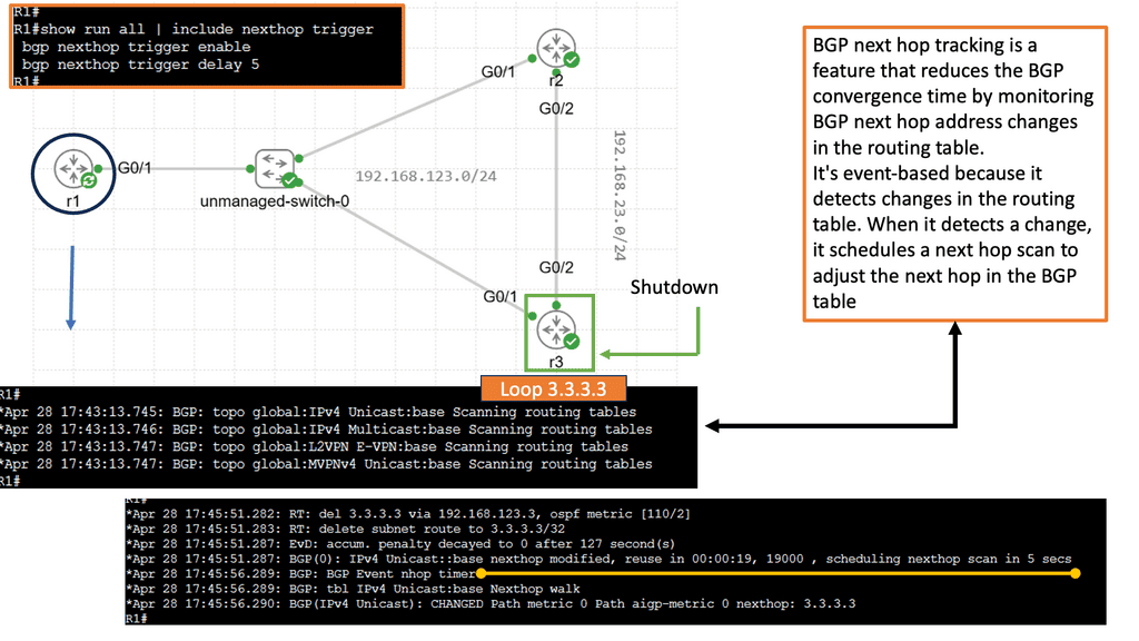
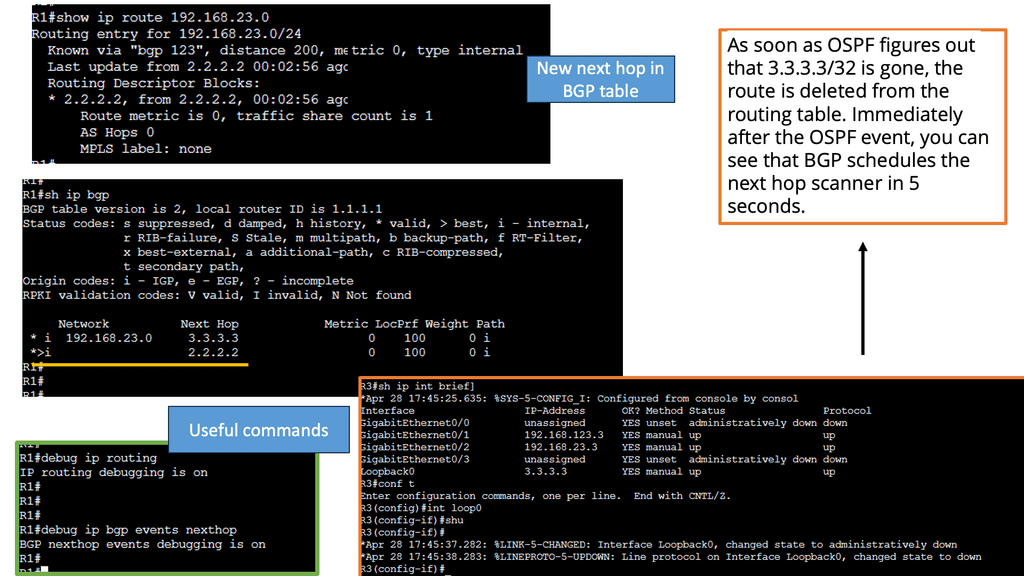
**Benefits of Efficient Routing Convergence:**
1. Improved Network Performance: Efficient routing convergence reduces network congestion, latency, and packet loss, improving overall network performance.
2. Enhanced Reliability: Routing convergence ensures uninterrupted communication and minimizes downtime by quickly adapting to changes in network conditions.
3. Scalability: Proper routing convergence techniques facilitate network expansion and accommodate increased traffic demands without sacrificing performance or reliability.
Example Technology: BFD
Bidirectional Forwarding Detection (BFD) is a lightweight protocol designed to detect failures in communication paths between routers or switches. It operates independently of the routing protocols and detects rapid failure by utilizing fast packet exchanges. Unlike traditional methods like hello packets, BFD offers sub-second detection, allowing quicker convergence and network stability. BFD is pivotal in achieving fast routing convergence, providing real-time detection, and facilitating swift rerouting decisions.
-Enhanced Network Resilience: By swiftly detecting link failures, BFD enables routers to act immediately, rerouting traffic through alternate paths. This proactive approach ensures minimal disruption and enhances network resilience, especially in environments where redundancy is critical.
-Reduced Convergence Time: BFD’s ability to detect failures within milliseconds significantly reduces the time required for converging routing protocols. This translates into improved network responsiveness, reduced packet loss, and enhanced user experience.
-Scalability and Flexibility: BFD can be implemented across various network topologies and routing protocols, making it a versatile solution. Whether a small enterprise network or a large-scale service provider environment, BFD adapts seamlessly, providing consistent performance and stability.
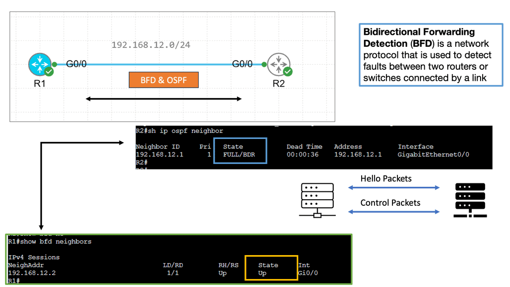
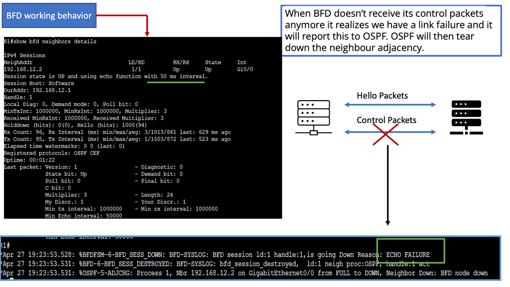
Convergence Time
Convergence time measures the speed at which a group of routers converges. Fast and reliable convergent routers are a significant performance indicator for routing protocols. The size of the network is also essential. A more extensive network will converge more slowly than a smaller one.
When a few routers are connected to RIP, a routing protocol that converges slowly, it can take several minutes for the network to converge. A triggered update for a new route can speed up RIP’s convergence, but a hold-down timer will slow flushing an existing route. OSPF is an example of a fast-convergence routing protocol. It is impossible to limit the speed at which OSPF routers can converge.
Unless specific hardware and configuration conditions are met, networks can never converge. “Flapping” interfaces (ones that frequently change between “up” and “down”) propagate conflicting information throughout the network, so routers cannot agree on the current state. Route aggregation can deprive certain parts of a network of detailed routing information, resulting in faster convergence of topological information.
Topological information
A set of routers in a network share the same topological information during convergence or routing convergence. Routing protocols exchange topology information between routers in a network. Routers in a network receive routing information when convergence is reached. Therefore, all routers know the network topology and optimal route in a converged network.
Any change in the network – for example, the failure of a device – affects convergence until all routers are informed of the change. The convergence time in a network is the time it takes for routers to achieve convergence after a topology change. In high-performance service provider networks, sensitive applications are run that require fast failover in case of failures. Several factors determine a network’s convergence rate:
- Devices detect route failures. Finding a new forwarding path begins with identifying the failed device. The existence of virtual networks establishes device reachability through their longevity, as opposed to physical networks, in which events determine device availability. To achieve fast network convergence, the detection time – the time it takes to detect a failure – must be kept within acceptable limits.
- In the event of a device failure on the primary route, traffic is diverted to the backup route. The failure or topology change has not yet affected all devices.
- Routing protocols are said to achieve global repair or network convergence when they propagate a change in topology to all network devices.
Understanding UDLD
UDLD, at its core, is a layer 2 protocol designed to detect and mitigate unidirectional links in Ethernet connections. It actively monitors the link status, allowing network devices to promptly detect and address potential issues. By verifying the bidirectional communication between neighboring devices, UDLD acts as a guardian, preventing one-way communication breakdowns.
Implementing UDLD brings forth numerous advantages for network administrators and organizations alike.
Firstly, it enhances network reliability by identifying and resolving unidirectional link failures that could otherwise lead to data loss and network disruptions.
Secondly, UDLD helps troubleshoot by providing valuable insights into link quality and integrity. This proactive approach aids in reducing downtime and improving overall network performance.
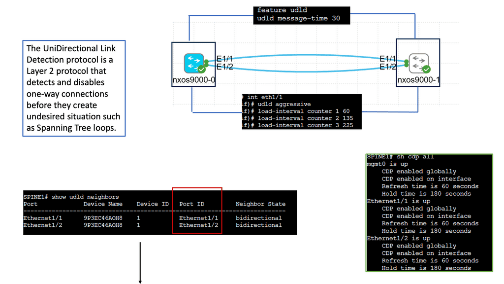
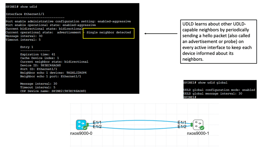
Enhancing Routing Convergence
Network administrators can implement various strategies to improve routing convergence. One approach is to utilize route summarization, which reduces the number of routes advertised and processed by routers. This helps minimize the impact of changes in specific network segments on overall convergence time.
Furthermore, implementing fast link failure detection mechanisms, such as Bidirectional Forwarding Detection (BFD), can significantly reduce convergence time. BFD allows routers to quickly detect link failures and trigger immediate updates to routing tables, ensuring faster convergence.
**Factors Influencing Routing Convergence**
Several factors impact routing convergence in a network. Firstly, the efficiency of the routing protocols being used plays a crucial role. Protocols such as OSPF (Open Shortest Path First) and EIGRP (Enhanced Interior Gateway Routing Protocol) are designed to facilitate fast convergence by quickly adapting to network changes.
Additionally, network topology and scale can affect routing convergence. Large networks with complex topologies may require more time for routers to converge due to the increased number of routes and potential link failures. Network administrators must carefully design and optimize the network architecture to minimize convergence time.
Control and data plane
When considering routing convergence with forwarding routing protocols, we must first highlight that a networking device is tasked with two planes of operation—the control plane and the data plane. The job of the data plane is to switch traffic across the router’s interfaces as fast as possible, i.e., move packets. The control plane has the more complex operation of putting together and creating the controls so the data plane can operate efficiently. How these two planes interact will affect network convergence time.
The network’s control plane finds the best path for routing convergence from any source to any network destination. For quick convergence routing, it must react quickly and dynamically to changes in the network, both on the LAN and on the WAN.
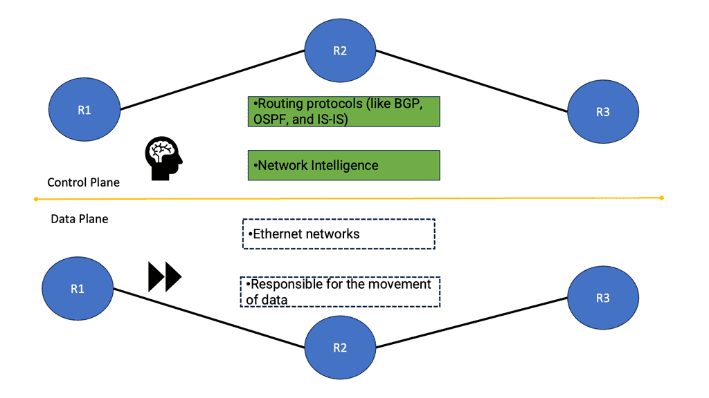
Monitoring and Troubleshooting Routing Convergence
Network administrators must monitor routing convergence to identify and promptly address potential issues. Network management tools, such as SNMP (Simple Network Management Protocol) and NetFlow analysis, can provide valuable insights into routing convergence performance, including convergence time, route flapping, and stability.
When troubleshooting routing convergence problems, administrators should carefully analyze routing table updates, link state information, and routing protocol logs. This information can help pinpoint the root cause of convergence delays or inconsistencies, allowing for targeted remediation.
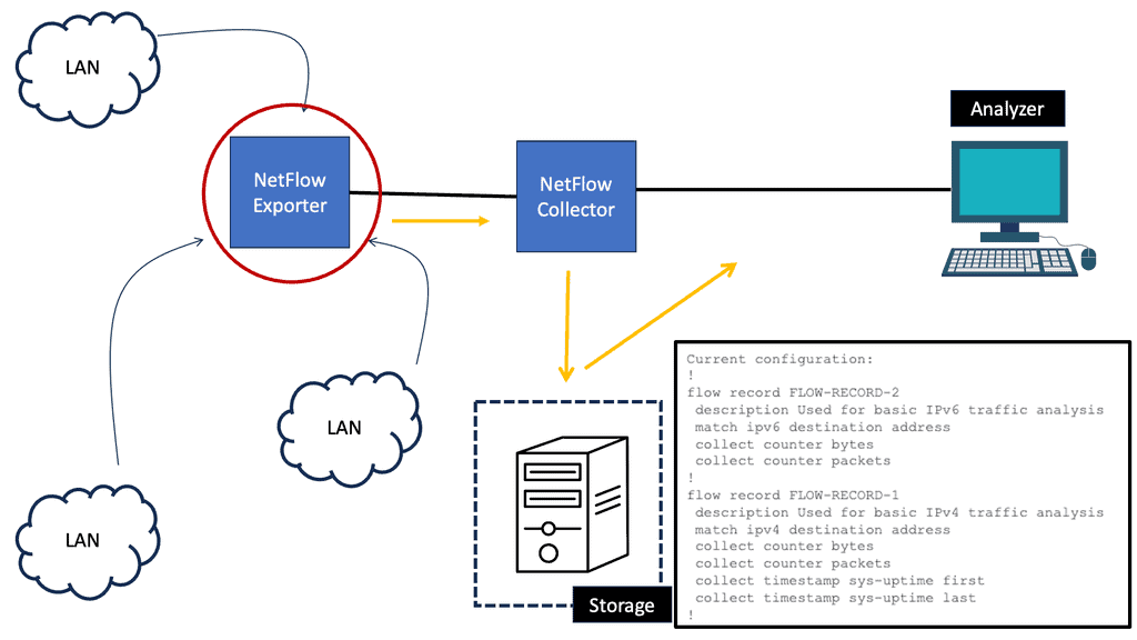
Related: For pre-information, you may find the following posts helpful:
Convergence Time Definition.
I found two similar definitions of convergence time:
“Convergence is the amount of time ( and thus packet loss ) after a failure in the network and before the network settles into a steady state.” Also, ” Convergence is the amount of time ( and thus packet loss) after a failure in the network and before the network responds to the failure.”
The difference between the two convergence time definitions is subtle but essential – steady-state vs. just responding. The control plane and its reaction to topology changes can be separated into four parts below. Each area must be addressed individually, as leaving one area out results in slow network convergence time and application time-out.
**IP routing**
Moving IP Packets
A router’s primary role is moving an IP packet from one network to another. Routers select the best loop-free path in a network to forward a packet to its destination IP address. A router learns about nonattached networks through static configuration or dynamic IP routing protocols. Both static and dynamic are examples of routing protocols.
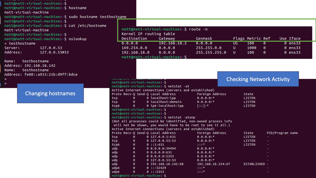
With dynamic IP routing protocols, we can handle network topology changes dynamically. Here, we can distribute network topology information between routers in the network. When there is a change in the network topology, the dynamic routing protocol provides updates without intervention when a topology change occurs.
On the other hand, we have IP routing to static routes, which do not accommodate topology changes very well and can be a burden depending on the network size. However, static routing is a viable solution for minimal networks with no modifications.
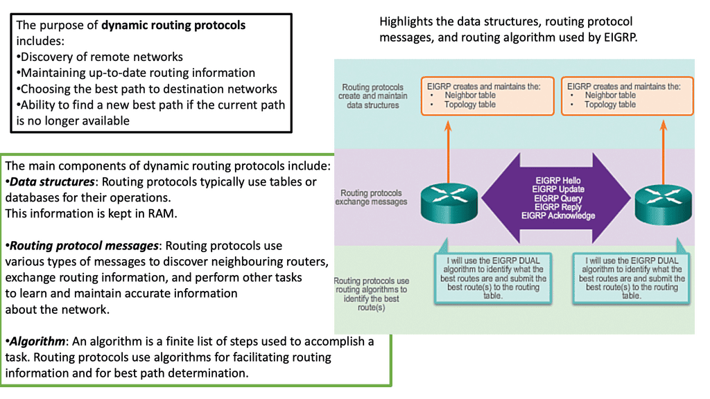
Knowledge Check: Bidirectional Forwarding Detection
Understanding BFD
BFD is a lightweight protocol designed to detect faults in the forwarding path between network devices. It operates at a low level, constantly monitoring the connectivity and responsiveness of neighboring devices. BFD can quickly detect failures by exchanging control packets and taking appropriate action to maintain network stability.
The Benefits of BFD
The implementation of BFD brings numerous advantages to network administrators and operators. Firstly, it provides rapid fault detection, reducing downtime and minimizing the impact of network failures. Additionally, BFD offers scalable and efficient operation, as it consumes minimal network resources. This makes it an ideal choice for large-scale networks where resource optimization is crucial.
BFD runs independently from other (routing) protocols. Once it’s up and running, you can configure protocols like OSPF, EIGRP, BGP, HSRP, MPLS LDP, etc., to use BFD for link failure detection instead of their mechanisms. When the link fails, BFD informs the protocol. When BFD no longer receives its control packets, it realizes we have a link failure and reports this to OSPF. OSPF will then tear down the neighbor adjacency.
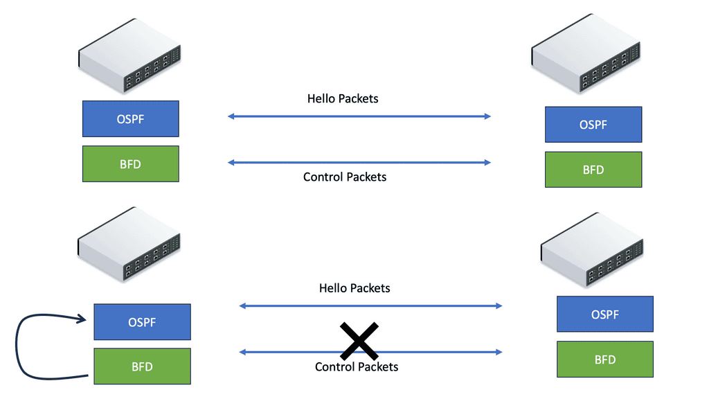
Use Cases of BFD
BFD finds its applications in various networking scenarios. One prominent use case is link aggregation, where BFD helps detect link failures and ensures seamless failover to alternate links. BFD is also widely utilized in Virtual Private Networks (VPNs) to monitor the connectivity of tunnel endpoints, enabling quick detection of connectivity issues and swift rerouting.
Implementing BFD in Practice
Implementing BFD requires careful consideration and configuration. Network devices must be appropriately configured to enable BFD sessions and define appropriate parameters such as timers and thresholds. Additionally, network administrators must ensure proper integration with underlying routing protocols to maximize BFD’s efficiency.
Convergence Routing and Network Convergence Time
Network convergence connects multiple computer systems, networks, or components to establish communication and efficient data transfer. However, it can be a slow process, depending on the size and complexity of the network, the amount of data that needs to be transferred, and the speed of the underlying technologies.
For networks to converge, all of the components must interact with each other and establish rules for data transfer. This process requires that the various components communicate with each other and usually involves exchanging configuration data to ensure that all components use the same protocols.
Network convergence is also dependent on the speed of the underlying technologies.
To speed up convergence, administrators should use the latest technologies, minimize the amount of data that needs to be transferred, and ensure that all components are correctly configured to be compatible. By following these steps, network convergence can be made faster and more efficient.
Example: OSPF
To put it simply, convergence or routing convergence is a state in which a set of routers in a network share the same topological information. For example, we have ten routers in one OSFP area. OSPF is an example of a fast-converging routing protocol. A network of a few OSPF routers can converge in seconds.
The routers within the OSPF area in the network collect the topology information from one another through the routing protocol. Depending on the routing protocol used to collect the data, the routers in the same network should have identical copies of routing information.
Different routing protocols will have additional convergence time. The time the routers take to reach convergence after a change in topology is termed convergence time. Fast network convergence and fast failover are critical factors in network performance. Before we get into the details of routing convergence, let us recap how networking works.
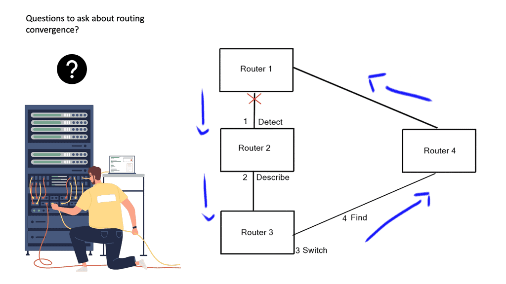
Unlike IS-IS, OSPF has fewer “knobs” for optimizing convergence. This is probably because IS-IS is being developed and supported by a separate team geared towards ISPs, where fast convergence is a competitive advantage.
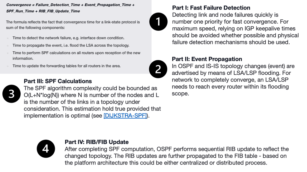
OSPF: Incremental SPF
OSPF calculates the SPT (Shortest Path Tree) using the SPF (Shortest Path First) algorithm. SPTs are built by OSPF routers within the same area with the same LSAs, LSDBs, and LSAs. OSPF routers will rerun a full SPF calculation even when there is just a single change in the network topology (change to an LSA type 1 and LSA type 2).
If a topology change occurs, we should run a full SPT calculation to find the shortest paths to all destinations. Unfortunately, we also calculate paths that have not changed since the last SPF.
In incremental SPF, OSPF only recalculates the parts of the SPT that have changed.
Because you don’t run a full SPF all the time, the router’s CPU load decreases,, and convergence times improve—additionally, your router stores the previous SPT copy, which requires more memory.
In three scenarios, incremental SPF is beneficial:
Adding (or removing) a leaf node to a branch
Link failure in non-SPT
Link failure in a branch of SPT
When many routers are in a single area, and the CPU load is high because of OSPF, incremental SPF can be enabled per router.
Forwarding Paradigms
We have bridging routing and switching with data and the control plane. So, we need to get packets across a network, which is easy if we have a single cable. You need to find the node’s address, and small and non-IP protocols would use a broadcast. When devices in the middle break this path, we can use source routing, path-based forwarding, and hop-by-hop address-based forwarding based solely on the destination address.
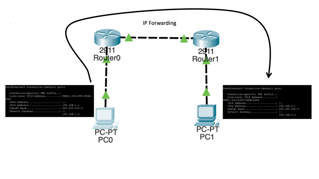
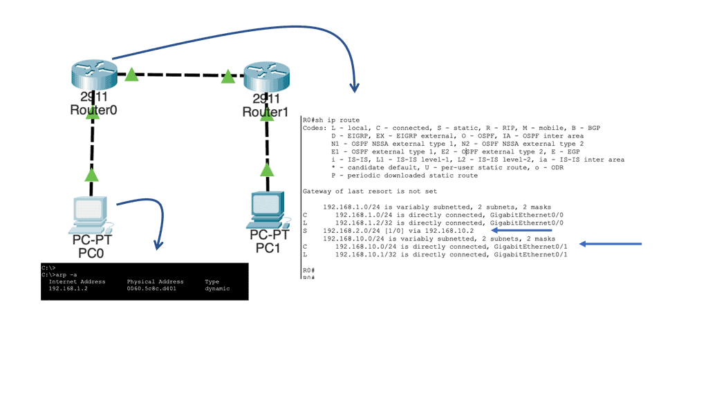
When protocols like IP came into play, hop-by-hop destination-based forwarding became the most popular; this is how IP forwarding works. Everyone in the path makes independent forwarding decisions. Each device looks at the destination address, examines its lookup tables, and decides where to send the packet.
**Finding paths across the network**
How do we find a path across the network? We know there are three ways to get packets across the network – source routing, path-based forwarding, and hop-by-hop destination-based forwarding. So, we need some way to populate the forwarding tables. You need to know how your neighbors are and who your endpoints are. This can be static routing, but it is more likely to be a routing protocol. Routing protocols have to solve and describe the routing convergence on the network at a high level.
When we are up and running, events can happen to the topology that force or make the routing protocols react and perform a convergence routing state. For example, we have a link failure, and the topology has changed, impacting our forwarding information. So, we must propagate the information and adjust the path information after the topology change. We know these convergence routing states are to detect, describe, switch, and find.
Rouitng Convergence | Convergence |
To better understand routing convergence, I would like to share the network convergence time for each routing protocol before diving into each step. The times displayed below are from a Cisco Live session based on real-world case studies and field research. We are separating each of the convergence routing steps described above into the following fields: Detect, describe, find alternative, and total time.
Routing Protocol | RIP | OSPF | EIGRP |
Detect | <1 second-best, 105 seconds average | <1 second-best, 20 seconds average | <1 second-best, 15 seconds average.30 seconds worst |
Describe | 15 seconds average, 30 seconds worst | 1 second-best, 5 seconds average. | 2 seconds |
Find Alternative | 15 seconds average, 30 seconds worst | 1-second average. | *** <500ms per query hop average Assume a 2-second average |
Total Time | Best Average Case: 31 seconds Average Case: 135 seconds Worse Case: 179 seconds | Best Average Case: 2 to 3 seconds Average Case: 25 seconds Worse Case: 45 seconds | Best Average Case: <1 second Average Case: 20 seconds Worse Case: 35 seconds |
*** The alternate route is found before the described phase due to the feasible successor design with EIGRP path selection.
Convergence Routing
Convergence routing: EIGPR
EIGRP is the fastest but only fractional. EIGRP has a pre-built loop-free path known as a feasible successor. The FS route has a higher metric than the successor, making it a backup route to the successor route. The effect of a pre-computed backup route on convergence is that EIGRP can react locally to a change in the network topology; nowadays, this is usually done in the FIB. EIGRP would have to query for the alternative route without a feasible successor, increasing convergence time.
However, you can have a Loop Free Alternative ( LFA ) for OSPF, which can have a pre-computed alternate path. Still, LFAs can only work with specific typologies and don’t guarantee against micro-loops ( EIGRP guarantees against micro-loops).
Lab Guide: EIGRP LFA FRR
With Loop-Free Alternate (LFA) Fast Reroute (FRR), EIGRP can switch to a backup path in less than 50 milliseconds. Fast rerouting means switching to another next hop, and a loop-free alternate refers to a loop-free alternative path.
Perhaps this sounds familiar to you. After all, EIGRP has feasible successors. The alternate paths calculated by EIGRP are loop-free. As soon as the successor fails, EIGRP can use a feasible successor.
It’s true, but there’s one big catch. In the routing table, EIGRP feasible successors are not immediately installed. Only one route is installed, the successor route. EIGRP installs the feasible successor when the successor fails, which takes time. By installing both successor routes and feasible successor routes in the routing table, fast rerouting makes convergence even faster.
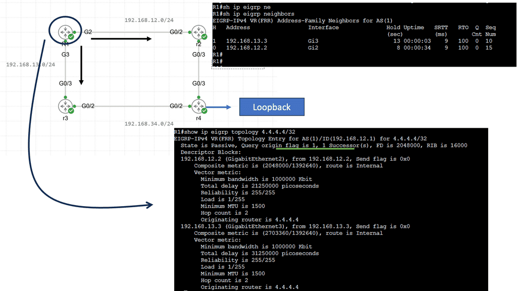
These four routers run EIGRP; there’s a loopback on R4 with network 4.4.4.4/32. R1 can go through R2 or R3 to get there. The delay on R1’s GigabitEthernet3 interface has increased, so R2 is our successor, and R3 is our feasible successor. The output below is interesting. We still see the successor route, but at the bottom, you can see the repair path…that’s our feasible successor.
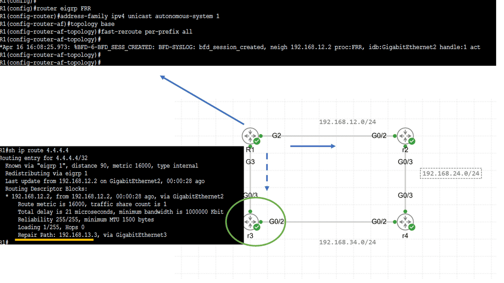
TCP Congestion control
Ask yourself, is < 1-second convergence fast enough for today’s applications? Indeed, the answer would be yes for some non-critical applications that work on TCP. TCP has built-in backoff algorithms that can deal with packet loss by re-transmitting to recover lost segments. However, non-bulk data applications like video and VOIP have stricter rules and require fast convergence and minimal packet loss.
For example, a 5-second delay in routing protocol convergence could mean several hundred dropped voice calls. A 50-second delay in a Gigabit Ethernet link implies about 6.25 GB of lost information.
Adding Resilience
To add resilience to a network, you can aim to make the network redundant. When you add redundancy, you are betting that outages of the original path and the backup path will not co-occur and that the primary path does not fate share with the backup path ( they do not share common underlying infrastructure, i.e., physical conducts or power ).
There needs to be a limit on the number of links you add to make your network redundant, and adding 50 extra links does not make your network 50 times more redundant. It does the opposite! The control plane is tasked with finding the best path and must react to modifications in the network as quickly as possible.
However, every additional link you add slows down the convergence of the router’s control plane as there is additional information to compute, resulting in longer convergence times. The correct number of backup links is a trade-off between redundancy versus availability. The optimal level of redundancy between two points should be two or three links. The fourth link would make the network converge slower.
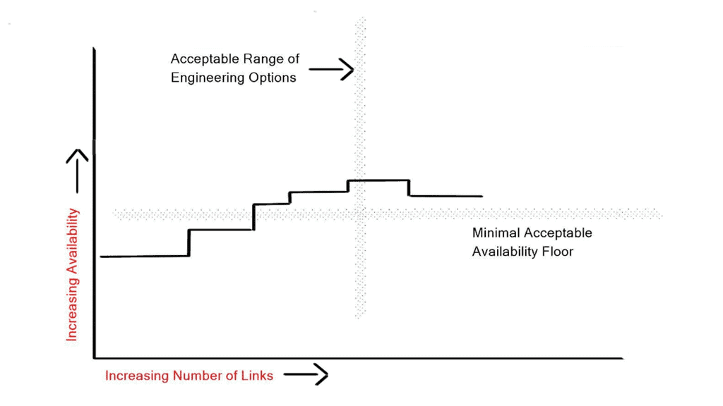
Routing Convergence and Routing Protocol Algorithms
Routing protocol algorithms can be tweaked to exponentially back off and deal with bulk information. However, no matter how many timers you use, the more data in the routing databases, the longer the convergence times. The primary way to reduce network convergence is to reduce the size of your routing tables by accepting just a default route, creating a flooding boundary domain, or using some other configuration method.
For example, a common approach in OSPF to reduce the size of routing tables and flooding boundaries is to create OSPF stub areas. OSPF stub areas limit the amount of information in the area. For example, EIGRP limits the flooding query domain by creating EIGRP stub routers and intelligently designing aggregation points. Now let us revisit the components of routing convergence:
Routing Convergence Step | Routing Convergence Details |
Step 1 | Failure detection |
Step 2 | Failure propagation ( flooding, etc.) IGP Reaction |
Step 3 | Topology/Routing calculation. IGP Reaction. |
Step 4 | Update the routing and forwarding table ( RIB & FIB) |
**Stage 1: Failure Detection**
The first and foremost problem facing the control plane is quickly detecting topology changes. Detecting the failure is the most critical and challenging part of network convergence. It can occur at different layers of the OSI stack – Physical Layers ( Layer 1), Data Link Layer ( Layer 2 ), Network Layer ( Layer 3 ), and Application layer ( Layer 7 ). There are many types of techniques used to detect link failures, but they all generally come down to two basic types:
- Event-driven notification occurs when a carrier is lost or when one network element detects a failure and notifies the other network elements.
- Polling-driven notification – generally HELLO protocols that test the path for reachability, such as Bidirectional Forwarding Detection ( BFD ). Event-driven notifications are always preferred over polling-driven ones as the latter have to wait for three polls before declaring a path down. However, there are some cases when you have multiple Layer devices in the path, and HELLO polling systems are the only method that can be used to detect a failure.
Layer 1 failure detection
Layer 1: Ethernet mechanisms like auto-negotiation ( 1 GigE ) and link fault signaling ( 10 GigE 802.3ae/ 40 GigE 802.3ba ) can signal local failures to the remote end.
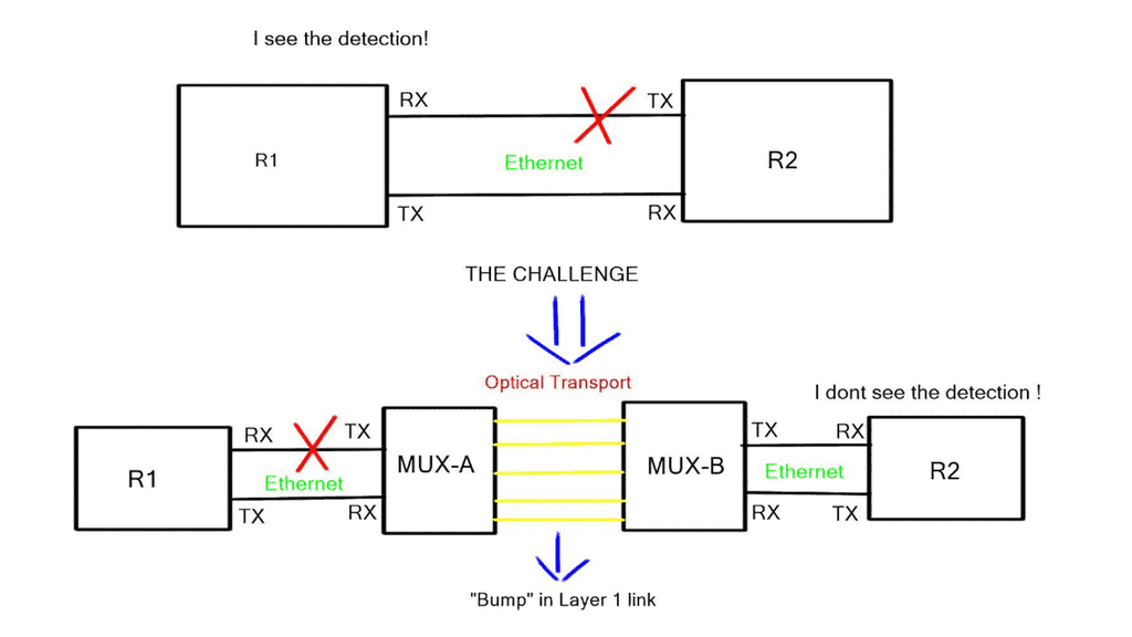
However, the challenge is getting the signal across an optical cloud, as relaying the fault information to the other end is impossible. When there is a “bump” in the Layer 1 link, it is not always possible for the remote end to detect the failure. In this case, the link fault signaling from Ethernet would get lost in the service provider’s network.
The actual link-down / interface-down event detection is hardware-dependent. Older platforms, such as the 6704 line cards for the Catalyst 6500, used a per-port polling mechanism, resulting in a 1 sec detect link failure period. More recent Nexus switches and the latest Catalyst 5600 line cards have an interrupt-driven notification mechanism resulting in high-speed and predictable link failure detection.
Layer 2 failure detection
Layer 2: The layer 2 detection mechanism will kick in if the Layer 1 mechanism does not. Unidirectional Link Detection ( UDLD ) is a Cisco proprietary lightweight Layer 2 failure detection protocol designed for detecting one-way connections due to physical or soft failure and miss-wirings.
- A key point: UDLD is a slow protocol
UDLD is a reasonably slow protocol that uses an average of 15 seconds for message interval and 21 seconds for detection. Its period has raised questions about its use in today’s data centers. However, the chances of miswirings are minimal; Layer 1 mechanisms always communicate unidirectional physical failure, and STP Bridge Assurance takes care of soft failures in either direction.
STP Bridge assurance turns STP into a bidirectional protocol and ensures that the spanning tree never fails to open and only fails to close. Failing open means that if a switch does not hear from its neighbor, it immediately starts forwarding on initially blocked ports, causing network havoc.
Layer 3 failure detection
Layer 3: In some cases, failure detection has to reply to HELLO protocols at Layer 3. This is needed when there are intermediate Layer 2 hops over Layer links and concerns over uni-direction failures on point-to-point physical links arise.
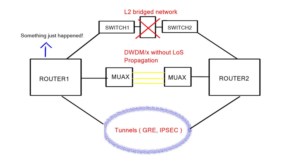
All Layer 3 protocols use HELLOs to maintain neighbor adjacency and a DEAD time to declare a neighbor dead. These timers can be tuned for faster convergence. However, it is generally not recommended due to the increase in CPU utilization causing false positives and the challenges ISSU and SSO face. They enable bidirectional forwarding detection ( BFD ) as the layer 3 detection mechanism is strongly recommended over aggressive protocol times, and they use BFD for all protocols.
Bidirectional Forwarding Detection ( BFD ) is a lightweight hello protocol for sub-second Layer 3 failure detection. It can run over multiple transport protocols, such as MPLS, THRILL, IPv6, and IPv4, making it the preferred method.
**Stage 2: Routing convergence and failure propagation**
When a change occurs in the network topology, it must be registered with the local router and transmitted throughout the rest of the network. The transmission of the change information will be carried out differently for Link-State and Distance Vector protocols. Link state protocols must flood information to every device in the network, and the distance vector must process the topology change at every hop through the network.
The processing of information at every hop may lead you to conclude that link-state protocols always converge more quickly than path-vector protocols, but this is not the case. EIGRP, due to its pre-computed backup path, will converge more rapidly than any link-state protocol.
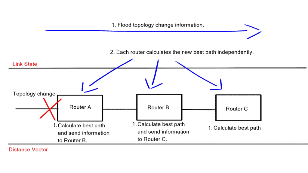
To propagate topology changes as quickly as possible, OSPF ( Link state ) can group changes into a few LSA while slowing down the rate at which information is flooded, i.e., do not flood on every change. This is accomplished with link-state flood timer tuning combined with exponential backoff systems, such as link-state advertisement delay / initial link-state advertisement throttle delay.
Unfortunately, Distance Vector Protocols do not have such timers. Therefore, reducing the routing table size is the only option for EIGRP. This can be done by aggregating and filtering reachability information ( summary route or Stub areas ).
**Stage 3: Topology/Routing calculation**
Similar to the second step, link-state protocols use exponential back-off timers in this step. These timers adjust the waiting time for OSPF and ISIS to wait after receiving new topology information before calculating the best path.
**Stage 4: Update the routing and forwarding table ( RIB & FIB)**
Finally, after the topology information has been flooding through the network and a new best path has been calculated, the new best path must be installed in the Forwarding Information Base ( FIB ). The FIB is a copy of the RIB in hardware, and the forwarding process finds it much easier to read than the RIB. However, again, this is usually done in hardware. Most vendors offer features that will install a pre-computed backup path on the line cards forwarding table so the fail-over from the primary path to the backup path can be done milliseconds without interrupting the router CPU.
Closing Points: Routing Convergence
Routing convergence refers to the process by which network routers exchange routing information and adapt to changes in network topology or routing policies. It involves the timely update and synchronization of routing tables across the network, allowing routers to determine the best paths for forwarding data packets.
Routing convergence is vital for maintaining network stability and minimizing disruptions. Network traffic may experience delays, bottlenecks, or even failures without proper convergence. Routing convergence enables efficient and reliable communication by ensuring all network routers have consistent routing information.
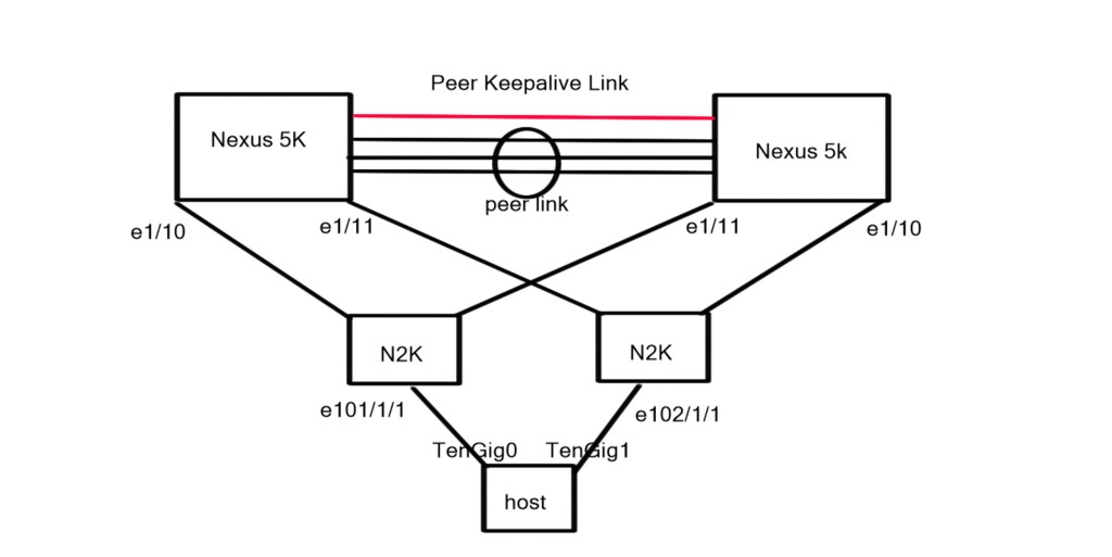
How-to: Fabric Extenders & VPC
Topology Diagram
The topology diagram depicts two Nexus 5K acting as parent switches with physical connections to two downstream Nexus 2k (FEX) acting as the 10G physical termination points for the connected server.

Part1. Connecting the FEX to the Parent switch:
The FEX and the parent switch use Satellite Discovery Protocol (SDP) periodic messages to discovery and register with one another.
When you initially log on to the Nexus 5K you can see that the OS does not recognise the FEX even though there are two FEXs that are cabled correctly to parent switch. As the FEX is recognised as a remote line card you would expect to see it with a “show module” command.
| N5K3# sh module Mod Ports Module-Type Model Status — —– ——————————– ———————- ———— 1 40 40x10GE/Supervisor N5K-C5020P-BF-SUP active * 2 8 8×1/2/4G FC Module N5K-M1008 ok Mod Sw Hw World-Wide-Name(s) (WWN) — ————– —— ————————————————– 1 5.1(3)N2(1c) 1.3 — 2 5.1(3)N2(1c) 1.0 93:59:41:08:5a:0c:08:08 to 00:00:00:00:00:00:00:00 Mod MAC-Address(es) Serial-Num — ————————————– ———- 1 0005.9b1e.82c8 to 0005.9b1e.82ef JAF1419BLMA 2 0005.9b1e.82f0 to 0005.9b1e.82f7 JAF1411AQBJ |
We issue the “feature fex” command we observe the FEX sending SDP messages to the parent switch i.e. RX but we don’t see the parent switch sending SDP messages to the FEX i.e. TX.
Notice in the output below there is only “fex:Sdp-Rx” messages.
| N5K3# debug fex pkt-trace N5K3# 2014 Aug 21 09:51:57.410701 fex: Sdp-Rx: Interface: Eth1/11, Fex Id: 0, Ctrl Vntag: -1, Ctrl Vlan: 1 2014 Aug 21 09:51:57.410729 fex: Sdp-Rx: Refresh Intvl: 3000ms, Uid: 0x4000ff2929f0, device: Fex, Remote link: 0x20000080 2014 Aug 21 09:51:57.410742 fex: Sdp-Rx: Vendor: Cisco Systems Model: N2K-C2232PP-10GE Serial: FOC17100NHX 2014 Aug 21 09:51:57.821776 fex: Sdp-Rx: Interface: Eth1/10, Fex Id: 0, Ctrl Vntag: -1, Ctrl Vlan: 1 2014 Aug 21 09:51:57.821804 fex: Sdp-Rx: Refresh Intvl: 3000ms, Uid: 0x2ff2929f0, device: Fex, Remote link: 0x20000080 2014 Aug 21 09:51:57.821817 fex: Sdp-Rx: Vendor: Cisco Systems Model: N2K-C2232PP-10GE Serial: FOC17100NHU |
The FEX appears as “DISCOVERED” but no additional FEX host interfaces appear when you issue a “show interface brief“.
Command: show fex [chassid_id [detail]]: Displays information about a specific Fabric Extender Chassis ID
Command: show interface brief: Display interface information and connection status for each interface.
| N5K3# sh fex FEX FEX FEX FEX Number Description State Model Serial ———————————————————————— — ——– Discovered N2K-C2232PP-10GE SSI16510AWF — ——– Discovered N2K-C2232PP-10GE SSI165204YC N5K3# N5K3# show interface brief ——————————————————————————– Ethernet VLAN Type Mode Status Reason Speed Port Interface Ch # ——————————————————————————– Eth1/1 1 eth access down SFP validation failed 10G(D) — Eth1/2 1 eth access down SFP validation failed 10G(D) — Eth1/3 1 eth access up none 10G(D) — Eth1/4 1 eth access up none 10G(D) — Eth1/5 1 eth access up none 10G(D) — Eth1/6 1 eth access down Link not connected 10G(D) — Eth1/7 1 eth access down Link not connected 10G(D) — Eth1/8 1 eth access down Link not connected 10G(D) — Eth1/9 1 eth access down Link not connected 10G(D) — Eth1/10 1 eth fabric down FEX not configured 10G(D) — Eth1/11 1 eth fabric down FEX not configured 10G(D) — Eth1/12 1 eth access down Link not connected 10G(D) — snippet removed |
The Fabric interface Ethernet1/10 show as DOWN with a “FEX not configured” statement.
| N5K3# sh int Ethernet1/10 Ethernet1/10 is down (FEX not configured) Hardware: 1000/10000 Ethernet, address: 0005.9b1e.82d1 (bia 0005.9b1e.82d1) MTU 1500 bytes, BW 10000000 Kbit, DLY 10 usec reliability 255/255, txload 1/255, rxload 1/255 Encapsulation ARPA Port mode is fex-fabric auto-duplex, 10 Gb/s, media type is 10G Beacon is turned off Input flow-control is off, output flow-control is off Rate mode is dedicated Switchport monitor is off EtherType is 0x8100 snippet removed |
To enable the parent switch to fully discover the FEX we need to issue the “switchport mode fex-fabric” under the connected interface. As you can see we are still not sending any SDP messages but we are discovering the FEX.
The next step is to enable the FEX logical numbering under the interface so we can start to configure the FEX host interfaces. Once this is complete we run the “debug fex pkt-trace” and we are not sending TX and receiving RX SDP messages.
Command:”fex associate chassis_id“: Associates a Fabric Extender (FEX) to a fabric interface. To disassociate the Fabric Extender, use the “no” form of this command.
From the “debug fexpkt-race” you can see the parent switch is now sending TX SDP messages to the fully discovered FEX.
| N5K3(config)# int Ethernet1/10 N5K3(config-if)# fex associate 101 N5K3# debug fex pkt-trace N5K3# 2014 Aug 21 10:00:33.674605 fex: Sdp-Tx: Interface: Eth1/10, Fex Id: 101, Ctrl Vntag: 0, Ctrl Vlan: 4042 2014 Aug 21 10:00:33.674633 fex: Sdp-Tx: Refresh Intvl: 3000ms, Uid: 0xc0821e9b0500, device: Switch, Remote link: 0x1a009000 2014 Aug 21 10:00:33.674646 fex: Sdp-Tx: Vendor: Model: Serial: ———- 2014 Aug 21 10:00:33.674718 fex: Sdp-Rx: Interface: Eth1/10, Fex Id: 0, Ctrl Vntag: 0, Ctrl Vlan: 4042 2014 Aug 21 10:00:33.674733 fex: Sdp-Rx: Refresh Intvl: 3000ms, Uid: 0x2ff2929f0, device: Fex, Remote link: 0x20000080 2014 Aug 21 10:00:33.674746 fex: Sdp-Rx: Vendor: Cisco Systems Model: N2K-C2232PP-10GE Serial: FOC17100NHU 2014 Aug 21 10:00:33.836774 fex: Sdp-Rx: Interface: Eth1/11, Fex Id: 0, Ctrl Vntag: -1, Ctrl Vlan: 1 2014 Aug 21 10:00:33.836803 fex: Sdp-Rx: Refresh Intvl: 3000ms, Uid: 0x4000ff2929f0, device: Fex, Remote link: 0x20000080 2014 Aug 21 10:00:33.836816 fex: Sdp-Rx: Vendor: Cisco Systems Model: N2K-C2232PP-10GE Serial: FOC17100NHX 2014 Aug 21 10:00:36.678624 fex: Sdp-Tx: Interface: Eth1/10, Fex Id: 101, Ctrl Vntag: 0, Ctrl Vlan: 4042 2014 Aug 21 10:00:36.678664 fex: Sdp-Tx: Refresh Intvl: 3000ms, Uid: 0xc0821e9b0500, device: Switch, Remote snippet removed |
Now the 101 FEX status changes from “DISCOVERED” to “ONLINE”. You may also see an additional FEX with serial number SSI165204YC as “DISCOVERED” and not “ONLINE”. This is due to the fact that we have not explicitly configured it under the other Fabric interface.
| N5K3# sh fex FEX FEX FEX FEX Number Description State Model Serial ———————————————————————— 101 FEX0101 Online N2K-C2232PP-10GE SSI16510AWF — ——– Discovered N2K-C2232PP-10GE SSI165204YC N5K3# N5K3# show module fex 101 FEX Mod Ports Card Type Model Status. — — —– ———————————- —————— ———– 101 1 32 Fabric Extender 32x10GE + 8x10G Module N2K-C2232PP-10GE present FEX Mod Sw Hw World-Wide-Name(s) (WWN) — — ————– —— ———————————————– 101 1 5.1(3)N2(1c) 4.4 — FEX Mod MAC-Address(es) Serial-Num — — ————————————– ———- 101 1 f029.29ff.0200 to f029.29ff.021f SSI16510AWF |
Issuing the “show interface brief” we see new interfaces, specifically host interfaces for the FEX. The syntax below shows that only one interface is up; interface labelled Eth101/1/1. Reason for this is that only one end host (server) is connected to the FEX
| N5K3# show interface brief ——————————————————————————– Ethernet VLAN Type Mode Status Reason Speed Port Interface Ch # ——————————————————————————– Eth1/1 1 eth access down SFP validation failed 10G(D) — Eth1/2 1 eth access down SFP validation failed 10G(D) — snipped removed ——————————————————————————– Port VRF Status IP Address Speed MTU ——————————————————————————– mgmt0 — up 192.168.0.53 100 1500 ——————————————————————————– Ethernet VLAN Type Mode Status Reason Speed Port Interface Ch # ——————————————————————————– Eth101/1/1 1 eth access up none 10G(D) — Eth101/1/2 1 eth access down SFP not inserted 10G(D) — Eth101/1/3 1 eth access down SFP not inserted 10G(D) — Eth101/1/4 1 eth access down SFP not inserted 10G(D) — Eth101/1/5 1 eth access down SFP not inserted 10G(D) — Eth101/1/6 1 eth access down SFP not inserted 10G(D) — snipped removed |
| N5K3# sh run int eth1/10 interface Ethernet1/10 switchport mode fex-fabric fex associate 101 |
The Fabric Interfaces do not run a Spanning tree instance while the host interfaces do run BPDU guard and BPDU filter by default. The reason why the fabric interfaces do not run spanning tree is because they are backplane point to point interfaces.
By default, the FEX interfaces will send out a couple of BPDU’s on start-up.
| N5K3# sh spanning-tree interface Ethernet1/10 No spanning tree information available for Ethernet1/10 N5K3# N5K3# N5K3# sh spanning-tree interface Eth101/1/1Vlan Role Sts Cost Prio.Nbr Type —————- —- — ——— ——– ——————————– VLAN0001 Desg FWD 2 128.1153 Edge P2p N5K3# N5K3# sh spanning-tree interface Eth101/1/1 detail Port 1153 (Ethernet101/1/1) of VLAN0001 is designated forwarding Port path cost 2, Port priority 128, Port Identifier 128.1153 Designated root has priority 32769, address 0005.9b1e.82fc Designated bridge has priority 32769, address 0005.9b1e.82fc Designated port id is 128.1153, designated path cost 0 Timers: message age 0, forward delay 0, hold 0 Number of transitions to forwarding state: 1 The port type is edge Link type is point-to-point by default Bpdu guard is enabled Bpdu filter is enabled by default BPDU: sent 11, received 0 |
| N5K3# sh spanning-tree interface Ethernet1/10 No spanning tree information available for Ethernet1/10 N5K3# N5K3# N5K3# sh spanning-tree interface Eth101/1/1Vlan Role Sts Cost Prio.Nbr Type—————- —- — ——— ——– ——————————– VLAN0001 Desg FWD 2 128.1153 Edge P2p N5K3# N5K3# sh spanning-tree interface Eth101/1/1 detail Port 1153 (Ethernet101/1/1) of VLAN0001 is designated forwarding Port path cost 2, Port priority 128, Port Identifier 128.1153 Designated root has priority 32769, address 0005.9b1e.82fc Designated bridge has priority 32769, address 0005.9b1e.82fc Designated port id is 128.1153, designated path cost 0 Timers: message age 0, forward delay 0, hold 0 Number of transitions to forwarding state: 1 The port type is edge Link type is point-to-point by default Bpdu guard is enabled Bpdu filter is enabled by default BPDU: sent 11, received 0 |
Issue the commands below to determine the transceiver type for the fabric ports and also the hosts ports for each fabric interface.
Command: “show interface fex-fabric“: displays all the Fabric Extender interfaces
Command: “show fex detail“: Shows detailed information about all FEXs. Including more recent log messages related to the FEX.
| N5K3# show interface fex-fabric Fabric Fabric Fex FEX Fex Port Port State Uplink Model Serial ————————————————————— 101 Eth1/10 Active 3 N2K-C2232PP-10GE SSI16510AWF — Eth1/11 Discovered 3 N2K-C2232PP-10GE SSI165204YC N5K3# N5K3# N5K3# show interface Ethernet1/10 fex-intf Fabric FEX Interface Interfaces ————————————————— Eth1/10 Eth101/1/1 N5K3# N5K3# show interface Ethernet1/10 transceiver Ethernet1/10 transceiver is present type is SFP-H10GB-CU3M name is CISCO-TYCO part number is 1-2053783-2 revision is N serial number is TED1530B11W nominal bitrate is 10300 MBit/sec Link length supported for copper is 3 m cisco id is — cisco extended id number is 4 N5K3# show fex detail FEX: 101 Description: FEX0101 state: Online FEX version: 5.1(3)N2(1c) [Switch version: 5.1(3)N2(1c)] FEX Interim version: 5.1(3)N2(1c) Switch Interim version: 5.1(3)N2(1c) Extender Serial: SSI16510AWF Extender Model: N2K-C2232PP-10GE, Part No: 73-12533-05 Card Id: 82, Mac Addr: f0:29:29:ff:02:02, Num Macs: 64 Module Sw Gen: 12594 [Switch Sw Gen: 21] post level: complete pinning-mode: static Max-links: 1 Fabric port for control traffic: Eth1/10 FCoE Admin: false FCoE Oper: true FCoE FEX AA Configured: false Fabric interface state: Eth1/10 – Interface Up. State: Active Fex Port State Fabric Port Eth101/1/1 Up Eth1/10 Eth101/1/2 Down None Eth101/1/3 Down None Eth101/1/4 Down None snippet removed Logs: 08/21/2014 10:00:06.107783: Module register received 08/21/2014 10:00:06.109935: Registration response sent 08/21/2014 10:00:06.239466: Module Online S |
Now we quickly enable the second FEX connected to fabric interface E1/11.
| N5K3(config)# int et1/11 N5K3(config-if)# switchport mode fex-fabric N5K3(config-if)# fex associate 102 N5K3(config-if)# end N5K3# sh fex FEX FEX FEX FEX Number Description State Model Serial ———————————————————————— 101 FEX0101 Online N2K-C2232PP-10GE SSI16510AWF 102 FEX0102 Online N2K-C2232PP-10GE SSI165204YC N5K3# show fex detail FEX: 101 Description: FEX0101 state: Online FEX version: 5.1(3)N2(1c) [Switch version: 5.1(3)N2(1c)] FEX Interim version: 5.1(3)N2(1c) Switch Interim version: 5.1(3)N2(1c) Extender Serial: SSI16510AWF Extender Model: N2K-C2232PP-10GE, Part No: 73-12533-05 Card Id: 82, Mac Addr: f0:29:29:ff:02:02, Num Macs: 64 Module Sw Gen: 12594 [Switch Sw Gen: 21] post level: complete pinning-mode: static Max-links: 1 Fabric port for control traffic: Eth1/10 FCoE Admin: false FCoE Oper: true FCoE FEX AA Configured: false Fabric interface state: Eth1/10 – Interface Up. State: Active Fex Port State Fabric Port Eth101/1/1 Up Eth1/10 Eth101/1/2 Down None Eth101/1/3 Down None Eth101/1/4 Down None Eth101/1/5 Down None Eth101/1/6 Down None snippet removed Logs: 08/21/2014 10:00:06.107783: Module register received 08/21/2014 10:00:06.109935: Registration response sent 08/21/2014 10:00:06.239466: Module Online Sequence 08/21/2014 10:00:09.621772: Module Online FEX: 102 Description: FEX0102 state: Online FEX version: 5.1(3)N2(1c) [Switch version: 5.1(3)N2(1c)] FEX Interim version: 5.1(3)N2(1c) Switch Interim version: 5.1(3)N2(1c) Extender Serial: SSI165204YC Extender Model: N2K-C2232PP-10GE, Part No: 73-12533-05 Card Id: 82, Mac Addr: f0:29:29:ff:00:42, Num Macs: 64 Module Sw Gen: 12594 [Switch Sw Gen: 21] post level: complete pinning-mode: static Max-links: 1 Fabric port for control traffic: Eth1/11 FCoE Admin: false FCoE Oper: true FCoE FEX AA Configured: false Fabric interface state: Eth1/11 – Interface Up. State: Active Fex Port State Fabric Port Eth102/1/1 Up Eth1/11 Eth102/1/2 Down None Eth102/1/3 Down None Eth102/1/4 Down None Eth102/1/5 Down None snippet removed Logs: 08/21/2014 10:12:13.281018: Module register received 08/21/2014 10:12:13.283215: Registration response sent 08/21/2014 10:12:13.421037: Module Online Sequence 08/21/2014 10:12:16.665624: Module Online |
Part 2. Fabric Interfaces redundancy
Static Pinning is when you pin a number of host ports to a fabric port. If the fabric port goes down so do the host ports that are pinned to it. This is useful when you want no oversubscription in the network.
Once the host port shut down due to a fabric port down event, the server if configured correctly should revert to the secondary NIC.
The “pinning max-link” divides the number specified in the command by the number of host interfaces to determine how many host interfaces go down if there is a fabric interface failure.
Now we shut down fabric interface E1/10, you can see that Eth101/1/1 has changed its operation mode to DOWN. The FEX has additional connectivity with E1/11 which remains up.
| Enter configuration commands, one per line. End with CNTL/Z. N5K3(config)# int et1/10 N5K3(config-if)# shu N5K3(config-if)# N5K3(config-if)# end N5K3# sh fex detail FEX: 101 Description: FEX0101 state: Offline FEX version: 5.1(3)N2(1c) [Switch version: 5.1(3)N2(1c)] FEX Interim version: 5.1(3)N2(1c) Switch Interim version: 5.1(3)N2(1c) Extender Serial: SSI16510AWF Extender Model: N2K-C2232PP-10GE, Part No: 73-12533-05 Card Id: 82, Mac Addr: f0:29:29:ff:02:02, Num Macs: 64 Module Sw Gen: 12594 [Switch Sw Gen: 21] post level: complete pinning-mode: static Max-links: 1 Fabric port for control traffic: FCoE Admin: false FCoE Oper: true FCoE FEX AA Configured: false Fabric interface state: Eth1/10 – Interface Down. State: Configured Fex Port State Fabric Port Eth101/1/1 Down Eth1/10 Eth101/1/2 Down None Eth101/1/3 Down None snippet removed Logs: 08/21/2014 10:00:06.107783: Module register received 08/21/2014 10:00:06.109935: Registration response sent 08/21/2014 10:00:06.239466: Module Online Sequence 08/21/2014 10:00:09.621772: Module Online 08/21/2014 10:13:20.50921: Deleting route to FEX 08/21/2014 10:13:20.58158: Module disconnected 08/21/2014 10:13:20.61591: Offlining Module 08/21/2014 10:13:20.62686: Module Offline Sequence 08/21/2014 10:13:20.797908: Module Offline FEX: 102 Description: FEX0102 state: Online FEX version: 5.1(3)N2(1c) [Switch version: 5.1(3)N2(1c)] FEX Interim version: 5.1(3)N2(1c) Switch Interim version: 5.1(3)N2(1c) Extender Serial: SSI165204YC Extender Model: N2K-C2232PP-10GE, Part No: 73-12533-05 Card Id: 82, Mac Addr: f0:29:29:ff:00:42, Num Macs: 64 Module Sw Gen: 12594 [Switch Sw Gen: 21] post level: complete pinning-mode: static Max-links: 1 Fabric port for control traffic: Eth1/11 FCoE Admin: false FCoE Oper: true FCoE FEX AA Configured: false Fabric interface state: Eth1/11 – Interface Up. State: Active Fex Port State Fabric Port Eth102/1/1 Up Eth1/11 Eth102/1/2 Down None Eth102/1/3 Down None Eth102/1/4 Down None snippet removed Logs: 08/21/2014 10:12:13.281018: Module register received 08/21/2014 10:12:13.283215: Registration response sent 08/21/2014 10:12:13.421037: Module Online Sequence 08/21/2014 10:12:16.665624: Module Online |
Port Channels can be used instead of static pinning between parent switch and FEX so in the event of a fabric interface failure all hosts ports remain active. However, the remaining bandwidth on the parent switch will be shared by all the host ports resulting in an increase in oversubscription.
Part 3. Fabric Extender Topologies
Straight-Through: The FEX is connected to a single parent switch. The servers connecting to the FEX can leverage active-active data plane by using host vPC.
Shutting down the Peer link results in ALL vPC member ports in the secondary peer become disabled. For this reason it is better to use a Dual Homed.
Dual Homed: Connecting a single FEX to two parent switches.
In active – active, a single parent switch failure does not affect the host’s interfaces because both vpc peers have separate control planes and manage the FEX separately.
For the remainder of the post we are going to look at Dual Homed FEX connectivity with host Vpc.
Full configuration:
| N5K1: feature lacp feature vpc feature fex ! vlan 10 ! vpc domain 1 peer-keepalive destination 192.168.0.52 ! interface port-channel1 switchport mode trunk spanning-tree port type network vpc peer-link ! interface port-channel10 switchport access vlan 10 vpc 10 ! interface Ethernet1/1 switchport access vlan 10 spanning-tree port type edge speed 1000 ! interface Ethernet1/3 – 5 switchport mode trunk spanning-tree port type network channel-group 1 mode active ! interface Ethernet1/10 switchport mode fex-fabric fex associate 101 ! interface Ethernet101/1/1 switchport access vlan 10 channel-group 10 mode on N5K2: feature lacp feature vpc feature fex ! vlan 10 ! vpc domain 1 peer-keepalive destination 192.168.0.51 ! interface port-channel1 switchport mode trunk spanning-tree port type network vpc peer-link ! interface port-channel10 switchport access vlan 10 vpc 10 ! interface Ethernet1/2 switchport access vlan 10 spanning-tree port type edge speed 1000 ! interface Ethernet1/3 – 5 switchport mode trunk spanning-tree port type network channel-group 1 mode active ! interface Ethernet1/11 switchport mode fex-fabric fex associate 102 ! interface Ethernet102/1/1 switchport access vlan 10 channel-group 10 mode on |
The FEX do not support LACP so configure the port-channel mode to “ON”
The first step is to check the VPC peer link and general VPC parameters.
Command: “show vpc brief“. Displays the vPC domain ID, the peer-link status, the keepalive message status, whether the configuration consistency is successful, and whether peer-link formed or the failure to form
Command: “show vpc peer-keepalive” Displays the destination IP of the peer keepalive message for the vPC. The command also displays the send and receives status as well as the last update from the peer in seconds and milliseconds
| N5K3# sh vpc brief Legend: (*) – local vPC is down, forwarding via vPC peer-link vPC domain id : 1 Peer status : peer adjacency formed ok vPC keep-alive status : peer is alive Configuration consistency status: success Per-vlan consistency status : success Type-2 consistency status : success vPC role : primary Number of vPCs configured : 1 Peer Gateway : Disabled Dual-active excluded VLANs : – Graceful Consistency Check : Enabled vPC Peer-link status ——————————————————————— id Port Status Active vlans — —- —— ————————————————– 1 Po1 up 1,10 vPC status —————————————————————————- id Port Status Consistency Reason Active vlans —— ———– —— ———– ————————– ———– 10 Po10 up success success 10 N5K3# show vpc peer-keepalive vPC keep-alive status : peer is alive –Peer is alive for : (1753) seconds, (536) msec –Send status : Success –Last send at : 2014.08.21 10:52:30 130 ms –Sent on interface : mgmt0 –Receive status : Success –Last receive at : 2014.08.21 10:52:29 925 ms –Received on interface : mgmt0 –Last update from peer : (0) seconds, (485) msec vPC Keep-alive parameters –Destination : 192.168.0.54 –Keepalive interval : 1000 msec –Keepalive timeout : 5 seconds –Keepalive hold timeout : 3 seconds –Keepalive vrf : management –Keepalive udp port : 3200 –Keepalive tos : 192 |
The trunk interface should be forwarding on the peer link and VLAN 10 must be forwarding and active on the trunk link. Take note if any vlans are on err-disable mode on the trunk.
| N5K3# sh interface trunk ——————————————————————————- Port Native Status Port Vlan Channel ——————————————————————————– Eth1/3 1 trnk-bndl Po1 Eth1/4 1 trnk-bndl Po1 Eth1/5 1 trnk-bndl Po1 Po1 1 trunking — ——————————————————————————– Port Vlans Allowed on Trunk ——————————————————————————– Eth1/3 1-3967,4048-4093 Eth1/4 1-3967,4048-4093 Eth1/5 1-3967,4048-4093 Po1 1-3967,4048-4093 ——————————————————————————– Port Vlans Err-disabled on Trunk ——————————————————————————– Eth1/3 none Eth1/4 none Eth1/5 none Po1 none ——————————————————————————– Port STP Forwarding ——————————————————————————– Eth1/3 none Eth1/4 none Eth1/5 none Po1 1,10 ——————————————————————————– Port Vlans in spanning tree forwarding state and not pruned ——————————————————————————– Eth1/3 — Eth1/4 — Eth1/5 — Po1 — ——————————————————————————– Port Vlans Forwarding on FabricPath ——————————————————————————– N5K3# sh spanning-tree vlan 10 VLAN0010 Spanning tree enabled protocol rstp Root ID Priority 32778 Address 0005.9b1e.82fc This bridge is the root Hello Time 2 sec Max Age 20 sec Forward Delay 15 sec Bridge ID Priority 32778 (priority 32768 sys-id-ext 10) Address 0005.9b1e.82fc Hello Time 2 sec Max Age 20 sec Forward Delay 15 sec Interface Role Sts Cost Prio.Nbr Type —————- —- — ——— ——– ——————————– Po1 Desg FWD 1 128.4096 (vPC peer-link) Network P2p Po10 Desg FWD 1 128.4105 (vPC) Edge P2p Eth1/1 Desg FWD 4 128.129 Edge P2p |
Check the Port Channel database and determine the status of the port channel
| N5K3# show port-channel database port-channel1 Last membership update is successful 3 ports in total, 3 ports up First operational port is Ethernet1/3 Age of the port-channel is 0d:00h:13m:22s Time since last bundle is 0d:00h:13m:18s Last bundled member is Ethernet1/5 Ports: Ethernet1/3 [active ] [up] * Ethernet1/4 [active ] [up] Ethernet1/5 [active ] [up] port-channel10 Last membership update is successful 1 ports in total, 1 ports up First operational port is Ethernet101/1/1 Age of the port-channel is 0d:00h:13m:20s Time since last bundle is 0d:00h:02m:42s Last bundled member is Ethernet101/1/1 Time since last unbundle is 0d:00h:02m:46s Last unbundled member is Ethernet101/1/1 Ports: Ethernet101/1/1 [on] [up] * |
To execute reachability tests, create an SVI on the first parent switch and run ping tests. You must first enable the feature set “feature interface-vlan”. The reason we create an SVI in VLAN 10 is because we need an interfaces to source our pings.
| N5K3# conf t Enter configuration commands, one per line. End with CNTL/Z. N5K3(config)# fea feature feature-set N5K3(config)# feature interface-vlan N5K3(config)# int vlan 10 N5K3(config-if)# ip address 10.0.0.3 255.255.255.0 N5K3(config-if)# no shu N5K3(config-if)# N5K3(config-if)# N5K3(config-if)# end N5K3# ping 10.0.0.3 PING 10.0.0.3 (10.0.0.3): 56 data bytes 64 bytes from 10.0.0.3: icmp_seq=0 ttl=255 time=0.776 ms 64 bytes from 10.0.0.3: icmp_seq=1 ttl=255 time=0.504 ms 64 bytes from 10.0.0.3: icmp_seq=2 ttl=255 time=0.471 ms 64 bytes from 10.0.0.3: icmp_seq=3 ttl=255 time=0.473 ms 64 bytes from 10.0.0.3: icmp_seq=4 ttl=255 time=0.467 ms — 10.0.0.3 ping statistics — 5 packets transmitted, 5 packets received, 0.00% packet loss round-trip min/avg/max = 0.467/0.538/0.776 ms N5K3# ping 10.0.0.10 PING 10.0.0.10 (10.0.0.10): 56 data bytes Request 0 timed out 64 bytes from 10.0.0.10: icmp_seq=1 ttl=127 time=1.874 ms 64 bytes from 10.0.0.10: icmp_seq=2 ttl=127 time=0.896 ms 64 bytes from 10.0.0.10: icmp_seq=3 ttl=127 time=1.023 ms 64 bytes from 10.0.0.10: icmp_seq=4 ttl=127 time=0.786 ms — 10.0.0.10 ping statistics — 5 packets transmitted, 4 packets received, 20.00% packet loss round-trip min/avg/max = 0.786/1.144/1.874 ms N5K3# |
Do the same tests on the second Nexus 5K.
| N5K4(config)# int vlan 10 N5K4(config-if)# ip address 10.0.0.4 255.255.255.0 N5K4(config-if)# no shu N5K4(config-if)# end N5K4# ping 10.0.0.10 PING 10.0.0.10 (10.0.0.10): 56 data bytes Request 0 timed out 64 bytes from 10.0.0.10: icmp_seq=1 ttl=127 time=1.49 ms 64 bytes from 10.0.0.10: icmp_seq=2 ttl=127 time=1.036 ms 64 bytes from 10.0.0.10: icmp_seq=3 ttl=127 time=0.904 ms 64 bytes from 10.0.0.10: icmp_seq=4 ttl=127 time=0.889 ms — 10.0.0.10 ping statistics — 5 packets transmitted, 4 packets received, 20.00% packet loss round-trip min/avg/max = 0.889/1.079/1.49 ms N5K4# ping 10.0.0.13 PING 10.0.0.13 (10.0.0.13): 56 data bytes Request 0 timed out Request 1 timed out Request 2 timed out Request 3 timed out Request 4 timed out — 10.0.0.13 ping statistics — 5 packets transmitted, 0 packets received, 100.00% packet loss N5K4# ping 10.0.0.3 PING 10.0.0.3 (10.0.0.3): 56 data bytes Request 0 timed out 64 bytes from 10.0.0.3: icmp_seq=1 ttl=254 time=1.647 ms 64 bytes from 10.0.0.3: icmp_seq=2 ttl=254 time=1.298 ms 64 bytes from 10.0.0.3: icmp_seq=3 ttl=254 time=1.332 ms 64 bytes from 10.0.0.3: icmp_seq=4 ttl=254 time=1.24 ms — 10.0.0.3 ping statistics — 5 packets transmitted, 4 packets received, 20.00% packet loss round-trip min/avg/max = 1.24/1.379/1.647 ms |
Shut down one of the FEX links to the parent and you see that the FEX is still reachable via the other link that is in the port channel bundle.
| N5K3# conf t Enter configuration commands, one per line. End with CNTL/Z. N5K3(config)# int Eth101/1/1 N5K3(config-if)# shu N5K3(config-if)# end N5K3# N5K3# N5K3# ping 10.0.0.3 PING 10.0.0.3 (10.0.0.3): 56 data bytes 64 bytes from 10.0.0.3: icmp_seq=0 ttl=255 time=0.659 ms 64 bytes from 10.0.0.3: icmp_seq=1 ttl=255 time=0.515 ms 64 bytes from 10.0.0.3: icmp_seq=2 ttl=255 time=0.471 ms 64 bytes from 10.0.0.3: icmp_seq=3 ttl=255 time=0.466 ms 64 bytes from 10.0.0.3: icmp_seq=4 ttl=255 time=0.465 ms — 10.0.0.3 ping statistics — 5 packets transmitted, 5 packets received, 0.00% packet loss round-trip min/avg/max = 0.465/0.515/0.659 ms |
If you would like to futher your knowlege on VPC and how it relates to Data Center toplogies and more specifically, Cisco’s Application Centric Infrastructure (ACI), you can check out my following training courses on Cisco ACI. Course 1: Design and Architect Cisco ACI, Course 2: Implement Cisco ACI, and Course 3: Troubleshooting Cisco ACI,

Data Center Design with Active Active design
The Role of Data Centers
An enterprise’s data center houses the computational power, storage, and applications needed to run its operations. All content is sourced or passed through the data center infrastructure in the IT architecture. Performance, resiliency, and scalability must be considered when designing the data center infrastructure.
Furthermore, the data center design should be flexible so that new services can be deployed and supported quickly. The many considerations required for such a design are port density, access layer uplink bandwidth, actual server capacity, and oversubscription.
A few short years ago, data centers were very different from what they are today. In a multi-cloud environment, virtual networks have replaced physical servers that support applications and workloads across pools of physical infrastructure. Nowadays, data exists across multiple data centers, the edge, and public and private clouds.
Communication between these locations must be possible in the on-premises and cloud data centers. Public clouds are also collections of data centers. In the cloud, applications use the cloud provider’s data center resources.
Redundant data centers
Redundant data centers are essentially two or more in different physical locations. This enables organizations to move their applications and data to another data center if they experience an outage. This also allows for load balancing and scalability, ensuring the organization’s services remain available.
Redundant data centers are generally located in geographically dispersed locations. This ensures that if one of the data centers experiences an issue, the other can take over, thus minimizing downtime. These data centers should also be connected via a high-speed network connection, such as a dedicated line or virtual private network, to allow seamless data transfers between the locations.
Implementing redundant data center BGP involves several crucial steps.
– Firstly, establishing a robust network architecture with multiple data centers interconnected via high-speed links is essential.
– Secondly, configuring BGP routers in each data center to exchange routing information and maintain consistent network topologies is crucial. Additionally, techniques such as Anycast IP addressing and route reflectors further enhance redundancy and fault tolerance.
**Benefits of Active-Active Data Center Design**
1. Enhanced Redundancy: With active-active design, organizations can achieve higher levels of redundancy by distributing the workload across multiple data centers. This redundancy ensures that even if one data center experiences a failure or maintenance downtime, the other data center seamlessly takes over, minimizing the impact on business operations.
2. Improved Performance and Scalability: Active-active design enables organizations to scale their infrastructure horizontally by distributing the load across multiple data centers. This approach ensures that the workload is evenly distributed, preventing any single data center from becoming a performance bottleneck. It also allows businesses to accommodate increasing demands without compromising performance or user experience.
3. Reduced Downtime: The active-active design significantly reduces the risk of downtime compared to traditional architectures. In the event of a failure, the workload can be immediately shifted to the remaining active data center, ensuring continuous availability of critical services. This approach minimizes the impact on end-users and helps organizations maintain their reputation for reliability.
4. Disaster Recovery Capabilities: Active-active data center design provides a robust disaster recovery solution. Organizations can ensure that their critical systems and applications remain operational despite a catastrophic failure at one location by having multiple geographically distributed data centers. This design approach minimizes the risk of data loss and provides a seamless failover mechanism.
**Implementation Considerations:**
Implementing an active-active data center design requires careful planning and consideration of various factors. Here are some key considerations:
1. Network Design: A robust and resilient network infrastructure is crucial for active-active data center design. Implementing load balancers, redundant network links, and dynamic routing protocols can help ensure seamless failover and optimal traffic distribution.
2. Data Synchronization: Organizations need to implement effective data synchronization mechanisms to maintain data consistency across multiple data centers. This may involve deploying real-time replication, distributed databases, or file synchronization protocols.
3. Application Design: Applications must be designed to be aware of the active-active architecture. They should be able to distribute the workload across multiple data centers and seamlessly switch between them in case of failure. Application-level load balancing and session management become critical in this context.
Active-active data center design offers organizations a robust solution for high availability and fault tolerance. Businesses can ensure uninterrupted access to critical systems and applications by distributing the workload across multiple data centers. The enhanced redundancy, improved performance, reduced downtime, and disaster recovery capabilities make active-active design an ideal choice for organizations striving to provide seamless and reliable services in today’s digital landscape.
Network Connectivity Center
### What is Google’s Network Connectivity Center?
Google Network Connectivity Center (NCC) is a centralized platform that enables enterprises to manage their global network connectivity. It integrates with Google Cloud’s global infrastructure, offering a unified interface to monitor, configure, and optimize network connections. Whether you are dealing with on-premises data centers, remote offices, or multi-cloud environments, NCC provides a streamlined approach to network management.
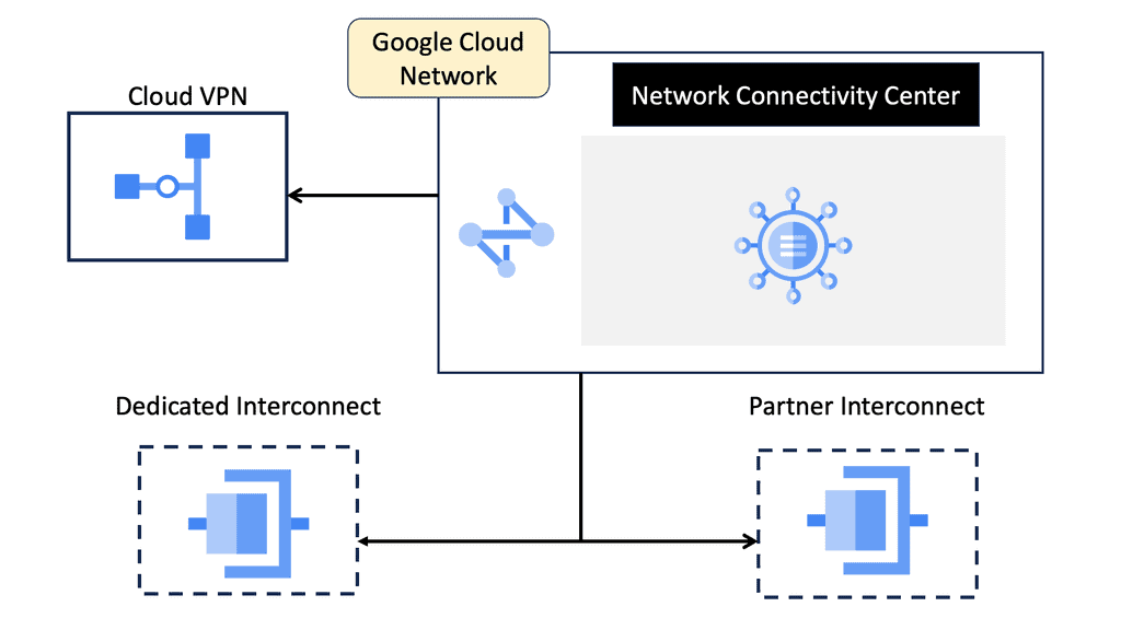
### Key Features of NCC
Google’s NCC is packed with features that make it an indispensable tool for network administrators. Here are some key highlights:
– **Centralized Management**: NCC offers a single pane of glass for monitoring and managing all network connections, reducing complexity and improving efficiency.
– **Scalability**: Built on Google Cloud’s robust infrastructure, NCC can scale effortlessly to accommodate growing network demands.
– **Automation and Intelligence**: With built-in automation and intelligent insights, NCC helps in proactive network management, minimizing downtime and optimizing performance.
– **Integration**: Seamlessly integrates with other Google Cloud services and third-party tools, providing a cohesive ecosystem for network operations.
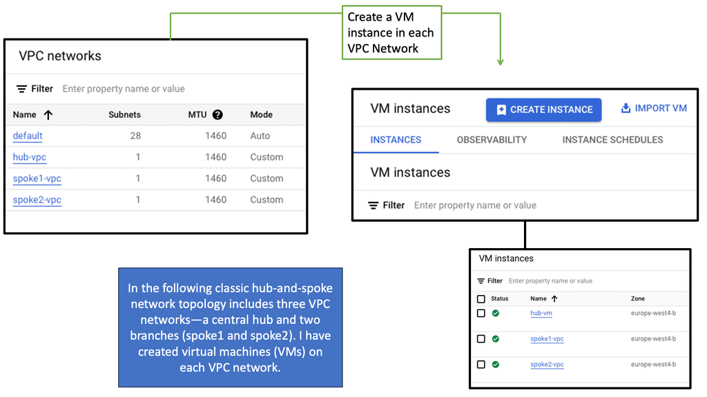
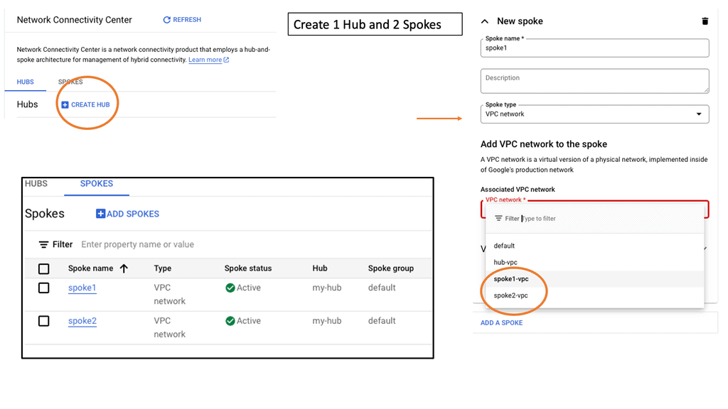
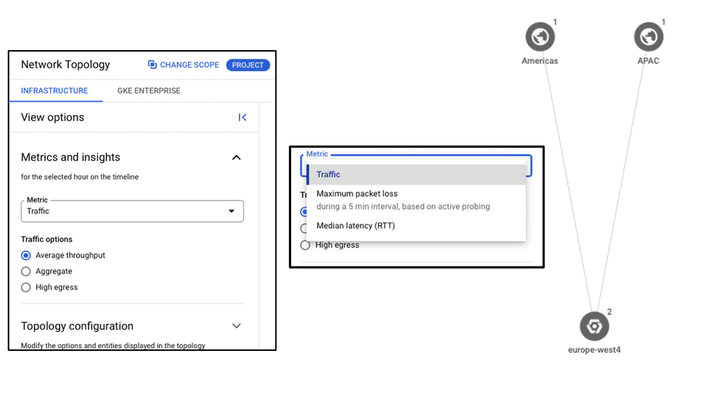
Understanding Network Tiers
Network tiers refer to the different levels of performance and cost offered by cloud service providers. They allow businesses to choose the most suitable network option based on their specific needs. Google Cloud offers two network tiers: Standard and Premium.
The Standard Tier provides businesses with a cost-effective network solution that meets their basic requirements. It offers reliable performance and ensures connectivity within Google Cloud services. With its lower costs, the Standard Tier is an excellent choice for businesses with moderate network demands.
For businesses that demand higher levels of performance and reliability, the Premium Tier is the way to go. This tier offers optimized routes, reduced latency, and enhanced global connectivity. With its advanced features, the Premium Tier ensures optimal network performance for mission-critical applications and services.
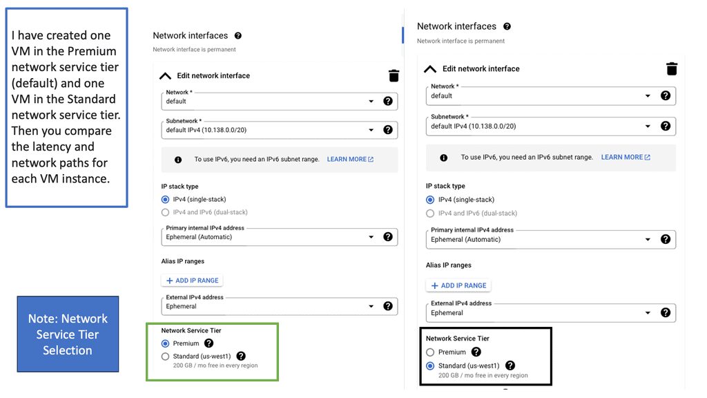
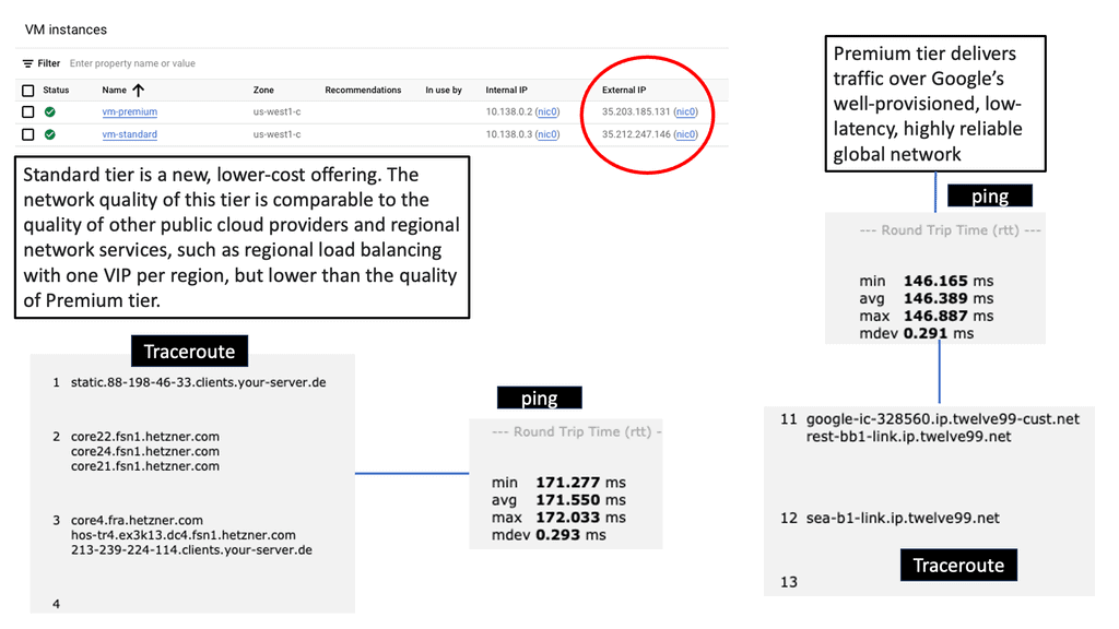
Understanding VPC Networking
VPC networking is the backbone of a cloud infrastructure, providing a private and secure environment for your resources. In Google Cloud, a VPC network can be thought of as your own virtual data center in the cloud. It allows you to define IP ranges, subnets, and firewall rules, empowering you with complete control over your network architecture.
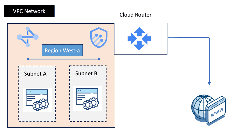
Google Cloud’s VPC networking offers a plethora of features that enhance network management and security. From custom IP address ranges to subnet creation and route configuration, you have the flexibility to design your network infrastructure according to your specific needs. Additionally, VPC peering and VPN connectivity options enable seamless communication with other networks, both within and outside of Google Cloud.
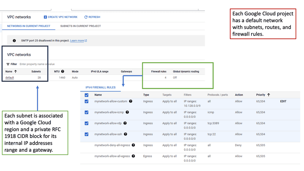
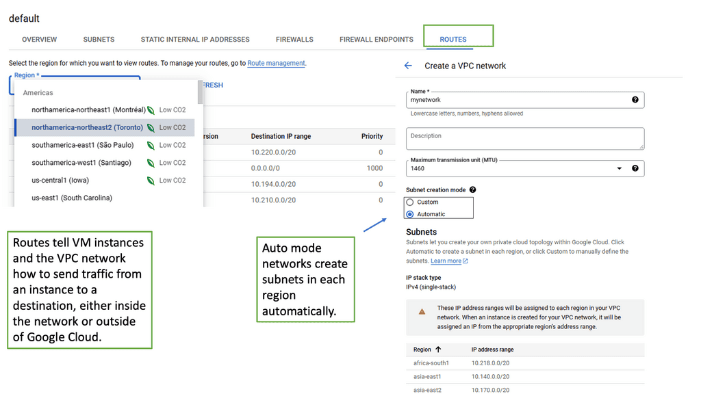 Understanding VPC Peering
VPC Peering enables you to connect VPC networks across projects or organizations. It allows for secure communication and seamless access to resources between peered networks. By leveraging VPC Peering, you can create a virtual network fabric across various environments.
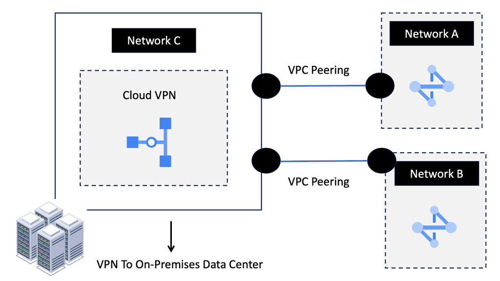
VPC Peering offers several advantages. First, it simplifies network architecture by eliminating the need for complex VPN setups or public IP addresses. Second, it provides low-latency and high-bandwidth connections between VPC networks, ensuring fast and reliable data transfer. Third, it lets you share resources across peering networks, such as databases or storage, promoting collaboration and resource optimization.
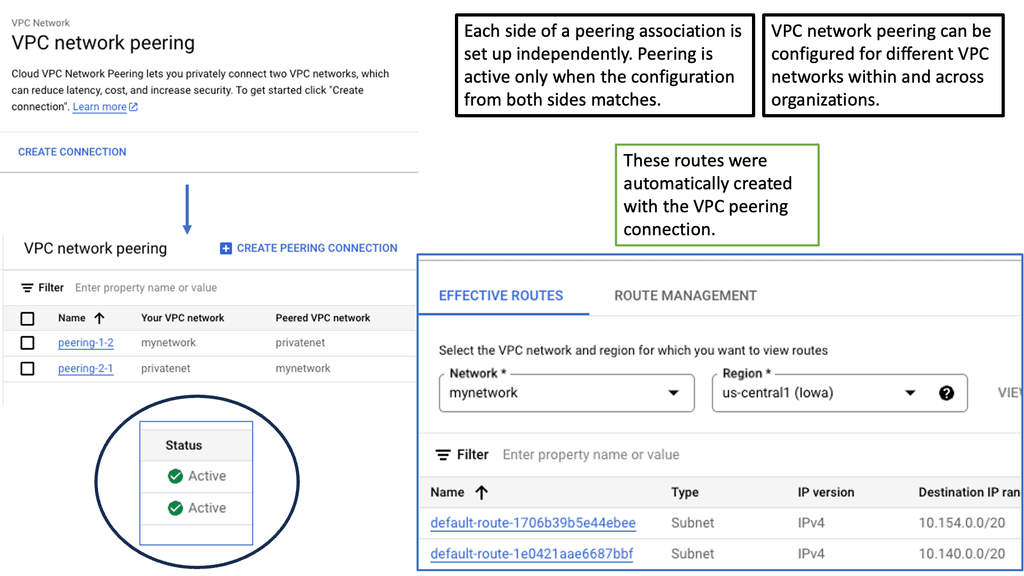
Understanding HA VPN
HA VPN, short for High Availability Virtual Private Network, is a feature provided by Google Cloud that ensures continuous and reliable connectivity between your on-premises network and your Google Cloud Virtual Private Cloud (VPC) network. It is designed to minimize downtime and provide fault tolerance by establishing redundant VPN tunnels.
To set up HA VPN, follow a few simple steps. First, ensure that you have a supported on-premises VPN gateway. Then, configure the necessary settings to create a VPN gateway in your VPC network. Next, configure the on-premises VPN gateway to establish a connection with the HA VPN gateway. Finally, validate the connectivity and ensure all traffic is routed securely through the VPN tunnels.
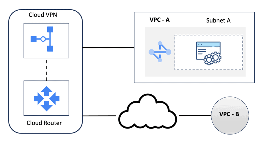
Implementing HA VPN offers several benefits for your network infrastructure. First, it enhances reliability by providing automatic failover in case of VPN tunnel or gateway failures, ensuring uninterrupted connectivity for your critical workloads. Second, HA VPN reduces the risk of downtime by offering a highly available and redundant connection. Third, it simplifies network management by centralizing the configuration and monitoring of VPN connections.
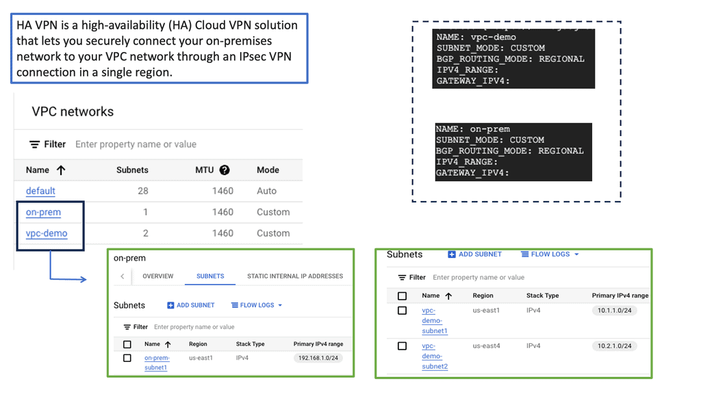
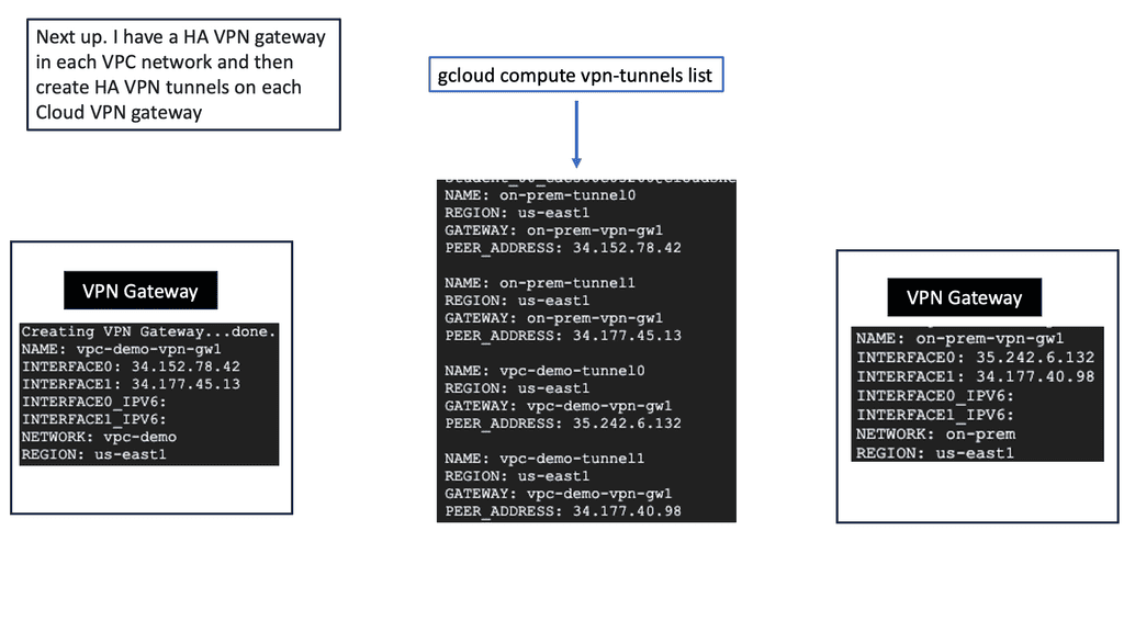 On-premises Data Centers
Understanding Nexus 9000 Series VRRP
Nexus 9000 Series VRRP is a protocol that allows multiple routers to work together as a virtual router, providing redundancy and seamless failover in the event of a failure. These routers ensure continuous network connectivity by sharing a virtual IP address, improving network reliability.
With Nexus 9000 Series VRRP, organizations can achieve enhanced network availability and minimize downtime. Utilizing multiple routers can eliminate single points of failure and maintain uninterrupted connectivity. This is particularly crucial in data center environments, where downtime can lead to significant financial losses and reputational damage.
Configuring Nexus 9000 Series VRRP involves several steps. First, a virtual IP address must be defined and assigned to the VRRP group. Next, routers participating in VRRP must be configured with their respective priority levels and advertisement intervals. Additionally, tracking mechanisms can monitor the availability of specific network interfaces and adjust the VRRP priority dynamically.
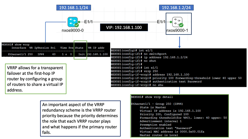
High Availability and BGP
High availability refers to the ability of a system or network to remain operational and accessible even during failures or disruptions. BGP is pivotal in achieving high availability by employing various mechanisms and techniques.
BGP Multipath is a feature that allows for the simultaneous use of multiple paths to reach a destination. BGP can use various paths to ensure redundancy, load balancing, and enhanced network availability.
BGP Route Reflectors are used in large-scale networks to alleviate the full-mesh requirement between BGP peers. By simplifying the BGP peering configuration, route reflectors enhance scalability and fault tolerance, contributing to high availability.
BGP Anycast is a technique that enables multiple servers or routers to share the same IP address. This method routes traffic to the nearest or least congested node, improving response times and fault tolerance.
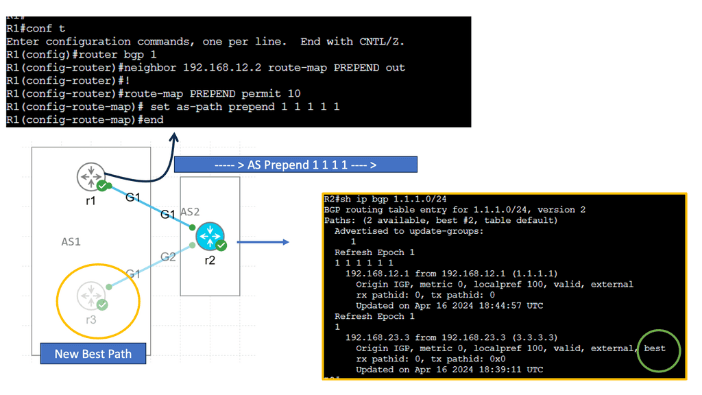
Understanding BGP Route Reflection
BGP route reflection is used in large-scale networks to reduce the number of full-mesh peerings required in a BGP network. It allows a BGP speaker to reflect routes received from one set of peers to another set of peers, eliminating the need for every peer to establish a direct connection with every other peer. Using route reflection, network administrators can simplify their network topology and improve its scalability.
The network must be divided into two main components to implement BGP route reflection: route reflectors and clients. Route reflectors serve as the central point for route reflection, while clients are the BGP speakers who establish peering sessions with the route reflectors. It is essential to carefully plan the placement of route reflectors to ensure optimal routing and redundancy in the network.
Route Reflector Hierarchy and Scaling
In large-scale networks, a hierarchy of route reflectors can be implemented to enhance scalability further. This involves using multiple route reflectors, where higher-level route reflectors reflect routes received from lower-level route reflectors. This hierarchical approach distributes the route reflection load and reduces the number of peering sessions required for each BGP speaker, thus improving scalability even further.
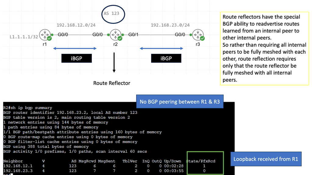
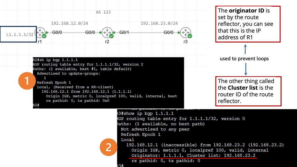
Understanding BGP Multipath
BGP multipath enables the selection and utilization of multiple equal-cost paths for forwarding traffic. Traditionally, BGP would only utilize a single best path, resulting in suboptimal network utilization. With multipath, network administrators can maximize link utilization, reduce congestion, and achieve load balancing across multiple paths.
One of the primary advantages of BGP multipath is enhanced network resilience. By utilizing multiple paths, networks become more fault-tolerant, as traffic can be rerouted in the event of link failures or congestion. Additionally, multipath can improve overall network performance by distributing traffic evenly across available paths, preventing bottlenecks, and ensuring efficient resource utilization.
Expansion and scalability
Expanding capacity is straightforward if a link is oversubscribed (more traffic than can be aggregated on the active link simultaneously). Expanding every leaf switch’s uplinks is possible, adding interlayer bandwidth and reducing oversubscription by adding a second spine switch. New leaf switches can be added by connecting them to every spine switch and configuring them as network switches if device port capacity becomes a concern. Scaling the network is made more accessible through ease of expansion. A nonblocking architecture can be achieved without oversubscription between the lower-tier switches and their uplinks.
Defining an active-active data center strategy isn’t easy when you talk to network, server, and compute teams that don’t usually collaborate when planning their infrastructure. An active-active Data center design requires a cohesive technology stack from end to end. Establishing the idea usually requires an enterprise-level architecture drive. In addition, it enables the availability and traffic load sharing of applications across DCs with the following use cases.
- Business continuity
- Mobility and load sharing
- Consistent policy and fast provisioning capability across
Understanding Spanning Tree Protocol (STP)
Spanning Tree Protocol (STP) is a fundamental mechanism to prevent loops in Ethernet networks. It ensures that only one active path exists between two network devices, preventing broadcast storms and data collisions. STP achieves this by creating a loop-free logical topology known as the spanning tree. But what about MST? Let’s find out.
As networks grow and become more complex, a single spanning tree may not be sufficient to handle the increasing traffic demands. This is where Spanning Tree MST comes into play. MST allows us to divide the network into multiple logical instances, each with its spanning tree. By doing so, we can distribute the traffic load more efficiently, achieving better performance and redundancy.
MST operates by grouping VLANs into multiple instances, known as regions. Each region has its spanning tree, allowing for independent configuration and optimization. MST relies on the concept of a Root Bridge, which acts as the central point for each instance. By assigning different VLANs to separate cases, we can control traffic flow and minimize the impact of network changes.
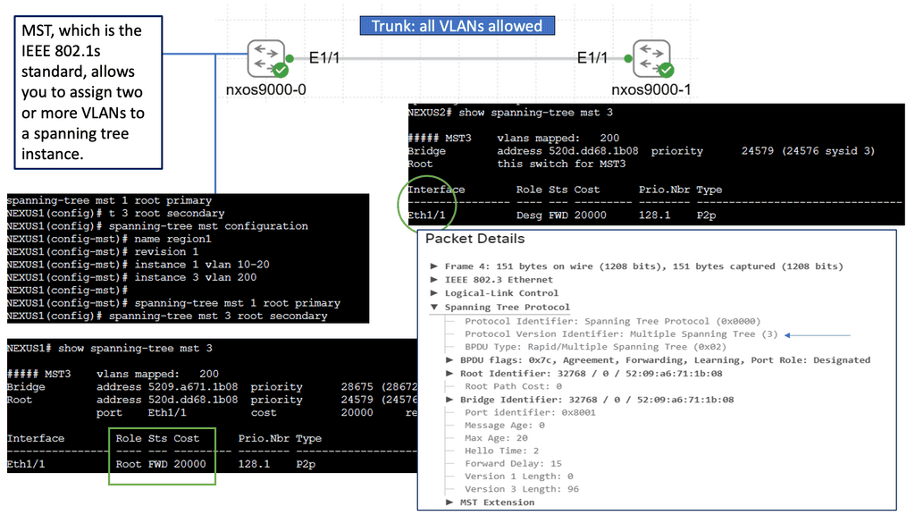
Example: Understanding UDLD
UDLD is a layer 2 protocol designed to detect and mitigate unidirectional links in a network. It operates by exchanging protocol packets between neighboring devices to verify the bidirectional nature of a link. UDLD prevents one-way communication and potential network disruptions by ensuring traffic flows in both directions.
UDLD helps maintain network reliability by identifying and addressing unidirectional links promptly. It allows network administrators to proactively detect and resolve potential issues before they can impact network performance. This proactive approach minimizes downtime and improves overall network availability.
Attackers can exploit unidirectional links to gain unauthorized access or launch malicious activities. UDLD acts as a security measure by ensuring bidirectional communication, making it harder for adversaries to manipulate network traffic or inject harmful packets. By safeguarding against such threats, UDLD strengthens the network’s security posture.
Understanding Port Channel
Port Channel, also known as Link Aggregation, is a mechanism that allows multiple physical links to be combined into a single logical interface. This logical interface provides higher bandwidth, improved redundancy, and load-balancing capabilities. Cisco Nexus 9000 Port Channel takes this concept to the next level, offering enhanced performance and flexibility.
a. Increased Bandwidth: By aggregating multiple physical links, the Cisco Nexus 9000 Port Channel significantly increases the available bandwidth, allowing for higher data throughput and improved network performance.
b. Redundancy and High Availability: Port Channel provides built-in redundancy, ensuring network resilience during link failures. With Cisco Nexus 9000, link-level redundancy is seamlessly achieved, minimizing downtime and maximizing network availability.
c. Load Balancing: Cisco Nexus 9000 Port Channel employs intelligent load balancing algorithms that distribute traffic across the aggregated links, optimizing network utilization and preventing bottlenecks.
d. Simplified Network Management: Cisco Nexus 9000 Port Channel simplifies network management by treating multiple links as a logical interface. This streamlines configuration, monitoring, and troubleshooting processes, leading to increased operational efficiency.
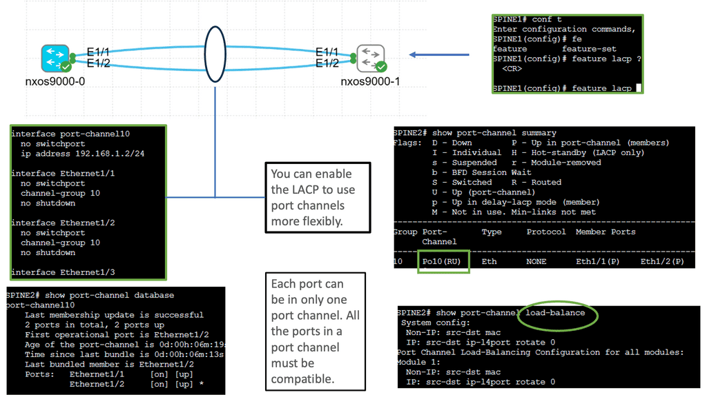
Understanding Virtual Port Channel (VPC)
VPC is a link aggregation technique that treats multiple physical links between two switches as a single logical link. This technology enables enhanced scalability, improved resiliency, and efficient utilization of network resources. By combining the bandwidth of multiple links, VPC provides higher throughput and creates a loop-free topology that eliminates the need for Spanning Tree Protocol (STP).
Implementing VPC brings several advantages to network administrators.
First, it enhances redundancy by providing seamless failover in case of link or switch failures.
Second, active-active multi-homing is achieved, ensuring traffic is evenly distributed across all available links.
Third, VPC simplifies network management by treating two switches as single entities, enabling streamlined configuration and consistent policy enforcement.
Lastly, VPC allows for the creation of large Layer 2 domains, facilitating workload mobility and flexibility.

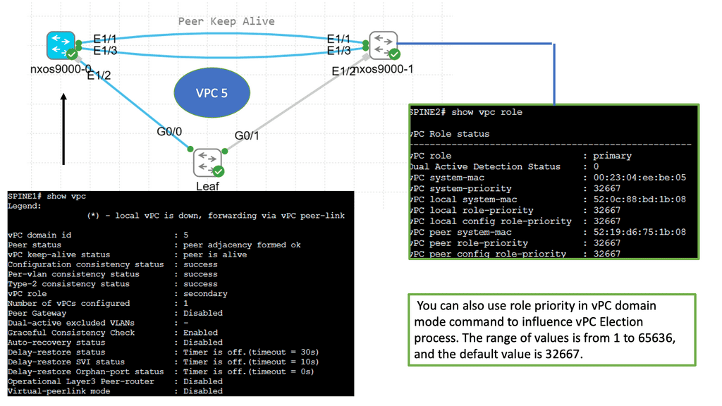
Understanding Nexus Switch Profiles
Nexus Switch Profiles are a feature of Cisco’s Nexus switches that enable administrators to define and manage a group of switch configurations as a single entity. This simplifies the management of complex networks by reducing manual configuration tasks and ensuring consistent settings across multiple switches. By encapsulating configurations into profiles, network administrators can achieve greater efficiency and operational agility.
Implementing Nexus Switch Profiles offers a plethora of benefits for network management. Firstly, it enables rapid deployment of new switches with pre-defined configurations, reducing time and effort. Secondly, profiles ensure consistency across the network, minimizing configuration errors and improving overall reliability. Additionally, profiles facilitate streamlined updates and changes, as modifications made to a profile are automatically applied to associated switches. This results in enhanced network security, reduced downtime, and simplified troubleshooting.
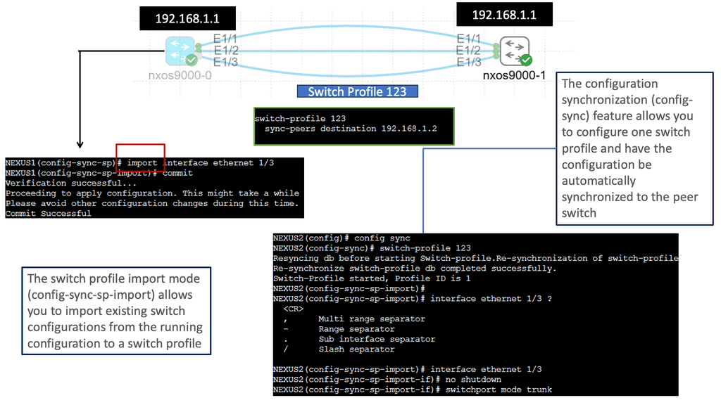
A. Active-active Transport Technologies
Transport technologies interconnect data centers. As part of the transport domain, redundancies and links are provided across the site to ensure HA and resiliency. Redundancy may be provided for multiplexers, GPONs, DCI network devices, dark fibers, diversity POPs for surviving POP failure, and 1+1 protection schemes for devices, cards, and links.
In addition, the following list contains the primary considerations to consider when designing a data center interconnection solution.
- Recovery from various types of failure scenarios: Link failures, module failures, node failures, etc.
- Traffic round-trip requirements between DCs based on link latency and applications
- Requirements for bandwidth and scalability
B. Active-Active Network Services
Network services connect all devices in data centers through traffic switching and routing functions. Applications should be able to forward traffic and share load without disruptions on the network. Network services also provide pervasive gateways, L2 extensions, and ingress and egress path optimization across the data centers. Most major network vendors’ SDN solutions also integrate VxLAN overlay solutions to achieve L2 extension, path optimization, and gateway mobility.
Designing active-active network services requires consideration of the following factors:
- Recovery from various failure scenarios, such as links, modules, and network devices, is possible.
- Availability of the gateway locally as well as across the DC infrastructure
- Using a VLAN or VxLAN between two DCs to extend the L2 domain
- Policies are consistent across on-premises and cloud infrastructure – including naming, segmentation rules for integrating various L4/L7 services, hypervisor integration, etc.
- Optimizing path ingresses and regresses.
- Centralized management includes inventory management, troubleshooting, AAA capabilities, backup and restore traffic flow analysis, and capacity dashboards.
C. Active-Active L4-L7 Services
ADC and security devices must be placed in both DCs before active-active L4-L7 services can be built. The major solutions in this space include global traffic managers, application policy controllers, load balancers, and firewalls. Furthermore, these must be deployed at different tiers for perimeter, extranet, WAN, core server farm, and UAT segments. Also, it should be noted that most of the leading L4-L7 service vendors currently offer clustering solutions for their products across the DCs. As a result of clustering, its members can share L4/L7 policies, traffic loads, and failover seamlessly in case of an issue.
Below are some significant considerations related to L4-L7 service design
- Various failure scenarios can be recovered, including link, module, and L4-L7 device failure.
- In addition to naming policies, L4-L7 rules for various traffic types must be consistent across the on-premises infrastructure and in the multiple clouds.
- Network management centralized (e.g., inventory, troubleshooting, AAA capabilities, backups, traffic flow analysis, capacity dashboards, etc.)
D. Active-Active Storage Services
Active-active data centers rely on storage and networking solutions. They refer to the storage in both DCs that serve applications. Similarly, the design should allow for uninterrupted read and write operations. Therefore, real-time data mirroring and seamless failover capabilities across DCs are also necessary. The following are some significant factors to consider when designing a storage system.
- Recover from single-disk failures, storage array failures, and split-brain failures.
- Asynchronous vs. synchronous replication: With synchronized replication, data is simultaneously written for primary storage and replica. It typically requires dedicated FC links, which consume more bandwidth.
- High availability and redundancy of storage: Storage replication factors and the number of disks available for redundancy
- Failure scenarios of storage networks: Links, modules, and network devices
E. Active-Active Server Virtualization
Over the years, server virtualization has evolved. Microservices and containers are becoming increasingly popular among organizations. The primary consideration here is to extend hypervisor/container clusters across the DCs to achieve seamless virtual machine/ container instance movement and fail-over. VMware Docker and Microsoft are the two dominant players in this market. Other examples include KVM, Kubernetes (container management), etc.
Here are some key considerations when it comes to virtualizing servers
- Creating a cross-DC virtual host cluster using a virtualization platform
- HA protects the VM in normal operational conditions and creates affinity rules that prefer local hosts.
- Deploying the same service, VMs in two DCs can take over the load in real time when the host machine is unavailable.
- A symmetric configuration with failover resources is provided across the compute node devices and DCs.
- Managing computing resources and hypervisors centrally
F. Active-Active Applications Deployment
The infrastructure needs to be in place for the application to function. Additionally, it is essential to ensure high application availability across DCs. Applications can also fail over and get proximity access to locations. It is necessary to have Web, App, and DB tiers available at both data centers, and if the application fails in one, it should allow fail-over and continuity.
Here are a few key points to consider
- Deploy the Web services on virtual or physical machines (VMs) by using multiple servers to form independent clusters per DC.
- VM or physical machine can be used to deploy App services. If the application supports distributed deployment, multiple servers within the DC can form a cluster or various servers across DCs can create a cluster (preferred IP-based access).
- The databases should be deployed on physical machines to form a cross-DC cluster (active-standby or active-active). For example, Oracle RAC, DB2, SQL with Windows server failover cluster (WSFC)
Knowledge Check: Default Gateway Redundancy
A first-hop redundancy protocol (FHRP) always provides an active default IP gateway. To transparently failover at the first-hop IP router, FHRPs use two or more routers or Layer 3 switches.
The default gateway facilitates network communication. Source hosts send data to their default gateways. Default gateways are IP addresses on routers (or Layer 3 switches) connected to the same subnet as the source hosts. End hosts are usually configured with a single default gateway IP address when the network topology changes. The local device cannot send packets off the local network segment if the default gateway is not reached. There is no dynamic method by which end hosts can determine the address of a new default gateway, even if there is a redundant router that may serve as the default gateway for that segment.
Advanced Topics:
Understanding VXLAN Flood and Learn
The flood and learning process is an essential component of VXLAN networks. It involves flooding broadcast, unknown unicast, and multicast traffic within the VXLAN segment to ensure that all relevant endpoints receive the necessary information. By using multicast, VXLAN optimizes network traffic and reduces unnecessary overhead.
Multicast plays a crucial role in enhancing the efficiency of VXLAN flood and learn. By utilizing multicast groups, the network can intelligently distribute traffic to only those endpoints that require the information. This approach minimizes unnecessary flooding, reduces network congestion, and improves overall performance.
Several components must be in place to enable VXLAN flood and learn with multicast. We will explore the necessary configurations on the VXLAN Tunnel Endpoints (VTEPs) and the underlying multicast infrastructure. Topics covered will include multicast group management, IGMP snooping, and PIM (Protocol Independent Multicast) configuration.
Related: Before you proceed, you may find the following useful:
At its core, an active active data center is based on fault tolerance, redundancy, and scalability principles. This means that the active data center should be designed to withstand any hardware or software failure, have multiple levels of data storage redundancy, and scale up or down as needed.
The data center also provides an additional layer of security. It is designed to protect data from unauthorized access and malicious attacks. It should also be able to detect and respond to any threats quickly and in a coordinated manner.
A comprehensive monitoring and management system is essential to ensure the data center functions correctly. This system should be designed to track the data center’s performance, detect problems, and provide the necessary alerting mechanisms. It should also provide insights into how the data center operates so that any necessary changes can be made.
Cisco Validated Design
Cisco has validated this design, which is freely available on the Cisco site. In summary, they have tested a variety of combinations, such as VSS-VSS, VSS-vPV, and vPC-vPC, and validated the design with 200 Layer 2 VLANs and 100 SVIs or 1000 VLANs and 1000 SVI with static routing.
At the time of writing, the M series for the Nexus 7000 supports native encryption of Ethernet frames through the IEEE 802.1AE standard. This implementation uses Advanced Encryption Standard ( AES ) cipher and a 128-bit shared key.
Example: Cisco ACI
In the following lab guide, we demonstrate Cisco ACI. To extend Cisco ACI, we have different designs, such as multi-site and multi-pod. This type of design overcomes many challenges of raising a data center, which we will discuss in this post, such as extending layer 2 networks.
One crucial value of the Cisco ACI is the COOP database that maps endpoints in the network. The following screenshots show the synchronized COOP database across spines, even in different data centers. Notice that the bridge domain VNID is mapped to the MAC address. The COOP database is unique to the Cisco ACI.
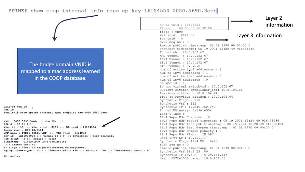
**The Challenge: Layer 2 is Weak**
The challenge of data center design is “Layer 2 is weak & IP is not mobile.” In the past, best practices recommended that networks from distinct data centers be connected through Layer 3 ( routing ), isolating the known Layer 2 turmoil. However, the business is driving the application requirements, changing the connectivity requirements between data centers.
The need for an active data center has been driven by the following. It is generally recommended to have Layer 3 connections with path separation through Multi-VRF, P2P VLANs, or MPLS/VPN, along with a modular building block data center design.
Yet, some applications cannot function over a Layer 3 environment. For example, most geo clusters require Layer 2 adjacency between their nodes, whether for heartbeat and connection ( status and control synchronization ) state information or the requirement to share virtual IP.
MAC addresses to facilitate traffic handling in case of failure. However, some clustering products ( Veritas, Oracle RAC ) support communication over Layer 3 but are a minority and don’t represent the general case.
Defining active data centers
The term active-active refers to using at least two data centers where both can service an application at any time, so each functions as an active application site. The demand for active-active data center architecture is to accomplish seamless workload mobility and enable distributed applications along with the ability to pool and maximize resources.
We must first have active-active data center infrastructure for an active/active application setup. Remember that the network is just one key component of active/active data centers). An active-active DC can be divided into two halves from a pure network perspective:-
- Ingress Traffic – inbound traffic
- Egress Traffic – outbound traffic
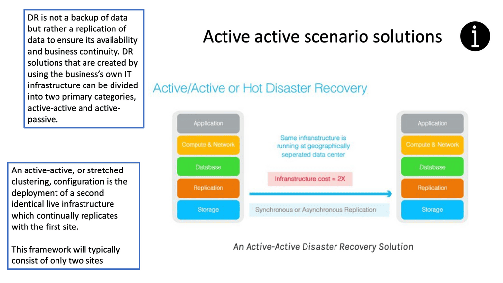
Active Active Data Center and VM Migration
Migrating applications and data to virtual machines (VMs) are becoming increasingly popular as organizations seek to reduce their IT costs and increase the efficiency of their services. VM migration moves existing applications, data, and other components from a physical server to a virtualized environment. This process is becoming increasingly more cost-effective and efficient for organizations, eliminating the need for additional hardware, software, and maintenance costs.
Virtual Machine migration between data centers increases application availability, Layer 2 network adjacency between ESX hosts is currently required, and a consistent LUN must be maintained for stateful migration. In other words, if the VM loses its IP address, it will lose its state, and the TCP sessions will drop, resulting in a cold migration ( VM does a reboot ) instead of a hot migration ( VM does not reboot ).
Due to the stretched VLAN requirement, data center architects started to deploy traditional Layer 2 over the DCI and, unsurprisingly, were faced with exciting results. Although flooding and broadcasts are necessary for IP communication in Ethernet networks, they can become dangerous in a DCI environment.
Traffic Tramboning
Traffic tromboning can also be formed between two stretched data centers, so nonoptimal internal routing happens within extended VLANs. Trombones, by their very nature, create a network traffic scalability problem. Addressing this through load balancing among multiple trombones is challenging since their services are often stateful.
Traffic tromboning can affect either ingress or egress traffic. On egress, you can have FHRP filtering to isolate the HSRP partnership and provide an active/active setup for HSRP. On ingress, you can have GSLB, Route Injection, and LISP.
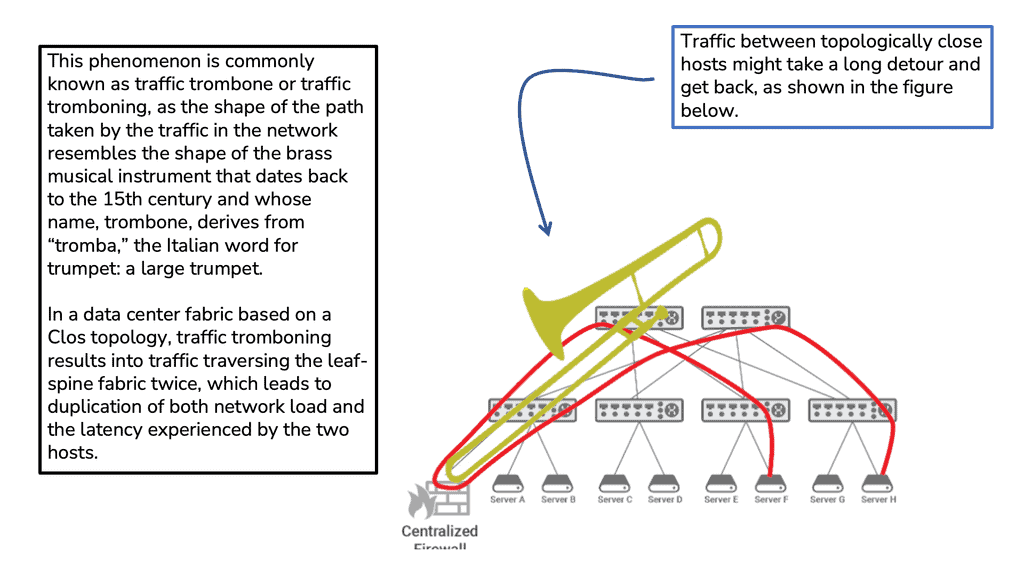
Cisco Active-active data center design and virtualization technologies
Virtualization technologies can overcome many of these problems by being used for Layer 2 extensions between data centers. These include vPC, VSS, Cisco FabricPath, VPLS, OTV, and LISP with its Internet locator design. In summary, different technologies can be used for LAN extensions, and the primary mediums in which they can be deployed are Ethernet, MPLS, and IP.
- Ethernet: VSS and vPC or Fabric Path
- MLS: EoMPLS and A-VPLS and H-VPLS
- IP: OTV
- LISP
Ethernet Extensions and Multi-Chassis EtherChannel ( MEC )
It requires protected DWDM or direct fibers and works only between two data centers. It cannot support multi-datacenter topology, i.e., a full mesh of data centers, but can help hub and spoke topologies.
Previously, LAG could only terminate on one physical switch. VSS-MEC and vPC are port-channeling concepts extending link aggregation to two physical switches. This allows for creating L2 typologies based on link aggregation, eliminating the dependency on STP, thus enabling you to scale available Layer 2 bandwidth by bonding the physical links.
Because vPC and VSS create a single connection from an STP perspective, disjoint STP instances can be deployed in each data center. Such isolation can be achieved with BPDU Filtering on the DCI links or Multiple Spanning Tree ( MST ) regions on each site.
At the time of writing, vPC does not support Layer 3 peering, but if you want an L3 link, create one, as this does not need to run on dark fiber or protected DWDM, unlike the extended Layer 2 links.
Ethernet Extension and Fabric path
The fabric path allows network operators to design and implement a scalable Layer 2 fabric, allowing VLANs to help reduce the physical constraints on server location. It provides a high-availability design with up to 16 active paths at layer 2, with each path a 16-member port channel for Unicast and Multicast.
This enables the MSDC networks to have flat typologies, separating nodes by a single hop ( equidistant endpoints ). Cisco has not targeted Fabric Path as a primary DCI solution as it does not have specific DCI functions compared to OTV and VPLS.
Its primary purpose is for Clos-based architectures. However, if you need to interconnect three or more sites, the Fabric path is a valid solution when you have short distances between your DCs via high-quality point-to-point optical transmission links.
Your WAN links must support Remote Port Shutdown and microflapping protection. By default, OTV and VPLS should be the first solutions considered as they are Cisco-validated designs with specific DCI features. For example, OTV can flood unknown unicast for particular VLANs.
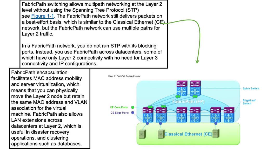
IP Core with Overlay Transport Virtualization ( OTV ).
OTV provides dynamic encapsulation with multipoint connectivity of up to 10 sites ( NX-OS 5.2 supports 6 sites, and NX-OS 6.2 supports 10 sites ). OTV, also known as Over-The-Top virtualization, is a specific DCI technology that enables Layer 2 extension across data center sites by employing a MAC in IP encapsulation with built-in loop prevention and failure boundary preservation.
There is no data plane learning. Instead, the overlay control plane ( Layer 2 IS-IS ) on the provider’s network facilitates all unicast and multicast learning between sites. OTV has been supported on the Nexus 7000 since the 5.0 NXOS Release and ASR 1000 since the 3.5 XE Release. OTV as a DCI has robust high availability, and most failures can be sub-sec convergence with only extreme and very unlikely failures such as device down resulting in <5 seconds.
Locator ID/Separator Protocol ( LISP)
Locator ID/Separator Protocol ( LISP) has many applications. As the name suggests, it separates the location and identifier of the network hosts, enabling VMs to move across subnet boundaries while retaining their IP address and enabling advanced triangular routing designs.
LISP works well when you have to move workloads and distribute workloads across data centers, making it a perfect complementary technology for an active-active data center design. It provides you with the following:
- a) Global IP mobility across subnets for disaster recovery and cloud bursting ( without LAN extension ) and optimized routing across extended subnet sites.
- b) Routing with extended subnets for active/active data centers and distributed clusters ( with LAN extension).
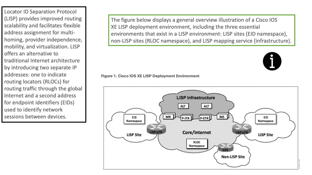
LISP answers the problems with ingress and egress traffic tromboning. It has a location mapping table, so when a host move is detected, updates are automatically triggered, and ingress routers (ITRs or PITRs) send traffic to the new location. From an ingress path flow inbound on the WAN perspective, LISP can answer our little problems with BGP in controlling ingress flows. Without LISP, we are limited to specific route filtering, meaning if you have a PI Prefix consisting of a /16.
If you break this up and advertise into 4 x /18, you may still get poor ingress load balancing on your DC WAN links; even if you were to break this up to 8 x /19, the results might still be unfavorable.
LISP works differently than BGP because a LISP proxy provider would advertise this /16 for you ( you don’t advertise the /16 from your DC WAN links ) and send traffic at 50:50 to our DC WAN links. LISP can get a near-perfect 50:50 conversion rate at the DC edge.