Understanding Convergence
Router convergence means they have the same topological information about the network they operate. To converge, a set of routers must have collected all topology information from each other using the routing protocol implemented. For this information to be accurate, it must reflect the current state of the network and not contradict other routers’ topology information.
All routers agree upon the topology of a converged network. For dynamic routing to work, a set of routers must be able to communicate with each other. All Interior Gateway Protocols depend on convergence. An autonomous system in operation is usually converged or convergent. Exterior Gateway Routing Protocol BGP rarely converges due to the size of the Internet.
Convergence Process
Each router in a routing protocol attempts to exchange topology information about the network. The extent, method, and type of information exchanged between routing protocols, such as BGP4, OSPF, and RIP, differs. A routing protocol convergence occurs once all routing protocol-specific information has been distributed to all routers. In the event of a routing table change in the network, convergence will be temporarily broken until the change has been successfully communicated to all routers.
Example: The convergence process
During the convergence process, routers exchange information about the network’s topology. Based on this information, they update their routing tables and calculate the most efficient paths to reach destination networks. This process continues until all routers have consistent and accurate routing tables.
The convergence time can vary depending on the size and complexity of the network and the routing protocols used. Convergence can happen relatively quickly in smaller networks, while more extensive networks may take longer to achieve convergence.
Network administrators can employ various strategies to optimize routing convergence. These include implementing fast convergence protocols, such as OSPF’s Fast Hello and Bidirectional Forwarding Detection (BFD), which minimize the time it takes to detect and respond to network changes.
Mechanisms for Achieving Routing Convergence:
1. Routing Protocols:
– Link-State Protocols: OSPF (Open Shortest Path First) and IS-IS (Intermediate System to Intermediate System) are examples of link-state protocols. They use flooding techniques to exchange information about network topology, allowing routers to calculate the shortest path to each destination.
– Distance-Vector Protocols: RIP (Routing Information Protocol) and EIGRP (Enhanced Interior Gateway Routing Protocol) are distance-vector protocols that use iterative algorithms to determine the best path based on distance metrics.
2. Fast Convergence Techniques:
– Triggered Updates: When a change occurs in network topology, routers immediately send updates to inform other routers about the change, reducing the convergence time.
– Route Flapping Detection: Route flapping occurs when a network route repeatedly becomes available and unavailable. By detecting and suppressing flapping routes, convergence time can be significantly improved.
– Convergence Optimization: Techniques like unequal-cost load balancing and route summarization help optimize routing convergence by distributing traffic across multiple paths and reducing the size of routing tables.
3. Redundancy and Resilience:
– Redundant Links: Multiple physical connections between routers increase network reliability and provide alternate paths in case of link failures.
– Virtual Router Redundancy Protocol (VRRP): VRRP allows multiple routers to act as a single virtual router, ensuring seamless failover in case of a primary router failure.
– Multi-Protocol Label Switching (MPLS): MPLS technology offers fast rerouting capabilities, enabling quick convergence in case of link or node failures.
Strategies for Achieving Optimal Routing Convergence
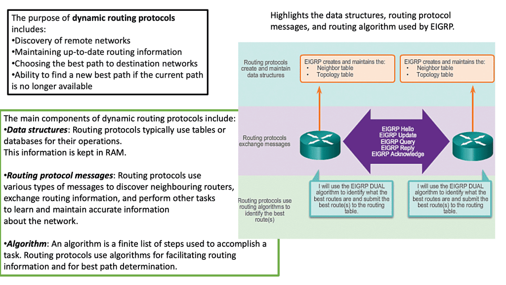
a. Enhanced Link-State Routing Protocol (EIGRP): EIGRP is a dynamic routing protocol that utilizes a Diffusing Update Algorithm (DUAL) to achieve fast convergence. By maintaining a backup route in case of link failures and employing triggered updates, EIGRP significantly reduces the time required for routing tables to converge.
b. Optimizing Routing Metrics: Carefully configuring routing metrics, such as bandwidth, delay, and reliability, can help achieve faster convergence. Assigning appropriate weights to these metrics ensures that routers quickly select the most efficient paths, leading to improved convergence times.
c. Implementing Route Summarization: Route summarization involves aggregating multiple network routes into a single summarized route. This technique reduces the size of routing tables and minimizes the complexity of route calculations, resulting in faster converge
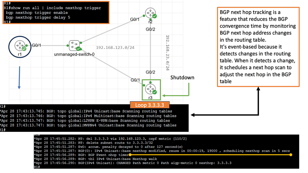
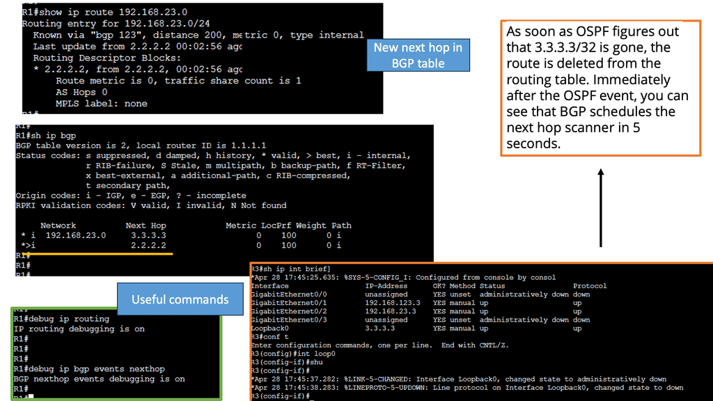
BGP Next Hop Tracking
BGP next hop refers to the IP address of the next router in the path towards a destination network. It serves as crucial information for routers to make forwarding decisions. Typically, BGP relies on the reachability of the next hop to determine the best path. However, various factors can affect this reachability, including link failures, network congestion, or misconfigurations. This is where BGP next hop tracking comes into play.
By incorporating next hop tracking into BGP, network administrators gain valuable insights into the reachability status of next hops. This information enables more informed decision-making regarding routing policies and traffic engineering. With real-time tracking, administrators can dynamically adjust routing paths based on the availability and quality of next hops, leading to improved network performance and reliability.
**Benefits of Efficient Routing Convergence:**
1. Improved Network Performance: Efficient routing convergence reduces network congestion, latency, and packet loss, improving overall network performance.
2. Enhanced Reliability: Routing convergence ensures uninterrupted communication and minimizes downtime by quickly adapting to changes in network conditions.
3. Scalability: Proper routing convergence techniques facilitate network expansion and accommodate increased traffic demands without sacrificing performance or reliability.
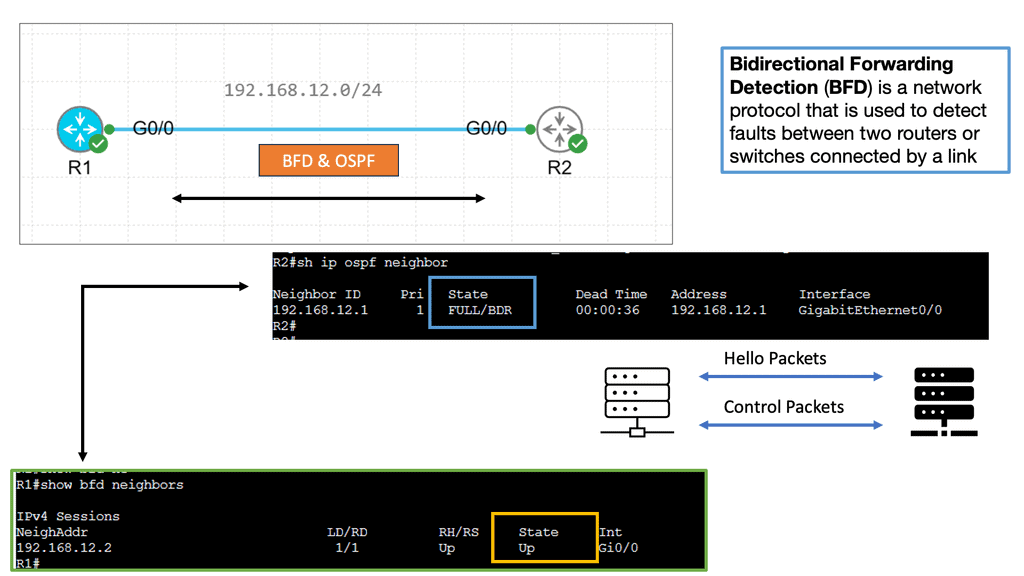
Example Technology: BFD
Bidirectional Forwarding Detection (BFD) is a lightweight protocol designed to detect failures in communication paths between routers or switches. It operates independently of the routing protocols and detects rapid failure by utilizing fast packet exchanges. Unlike traditional methods like hello packets, BFD offers sub-second detection, allowing quicker convergence and network stability. BFD is pivotal in achieving fast routing convergence, providing real-time detection, and facilitating swift rerouting decisions.
-Enhanced Network Resilience: By swiftly detecting link failures, BFD enables routers to act immediately, rerouting traffic through alternate paths. This proactive approach ensures minimal disruption and enhances network resilience, especially in environments where redundancy is critical.
-Reduced Convergence Time: BFD’s ability to detect failures within milliseconds significantly reduces the time required for converging routing protocols. This translates into improved network responsiveness, reduced packet loss, and enhanced user experience.
-Scalability and Flexibility: BFD can be implemented across various network topologies and routing protocols, making it a versatile solution. Whether a small enterprise network or a large-scale service provider environment, BFD adapts seamlessly, providing consistent performance and stability.
Convergence Time
Convergence time measures the speed at which a group of routers converges. Fast and reliable convergent routers are a significant performance indicator for routing protocols. The size of the network is also essential. A more extensive network will converge more slowly than a smaller one.
When a few routers are connected to RIP, a routing protocol that converges slowly, it can take several minutes for the network to converge. A triggered update for a new route can speed up RIP’s convergence, but a hold-down timer will slow flushing an existing route. OSPF is an example of a fast-convergence routing protocol. It is impossible to limit the speed at which OSPF routers can converge.
Unless specific hardware and configuration conditions are met, networks can never converge. “Flapping” interfaces (ones that frequently change between “up” and “down”) propagate conflicting information throughout the network, so routers cannot agree on the current state. Route aggregation can deprive certain parts of a network of detailed routing information, resulting in faster convergence of topological information.
Topological information
A set of routers in a network share the same topological information during convergence or routing convergence. Routing protocols exchange topology information between routers in a network. Routers in a network receive routing information when convergence is reached. Therefore, all routers know the network topology and optimal route in a converged network.
Any change in the network – for example, the failure of a device – affects convergence until all routers are informed of the change. The convergence time in a network is the time it takes for routers to achieve convergence after a topology change. In high-performance service provider networks, sensitive applications are run that require fast failover in case of failures. Several factors determine a network’s convergence rate:
- Devices detect route failures. Finding a new forwarding path begins with identifying the failed device. The existence of virtual networks establishes device reachability through their longevity, as opposed to physical networks, in which events determine device availability. To achieve fast network convergence, the detection time – the time it takes to detect a failure – must be kept within acceptable limits.
- In the event of a device failure on the primary route, traffic is diverted to the backup route. The failure or topology change has not yet affected all devices.
- Routing protocols are said to achieve global repair or network convergence when they propagate a change in topology to all network devices.
Understanding UDLD
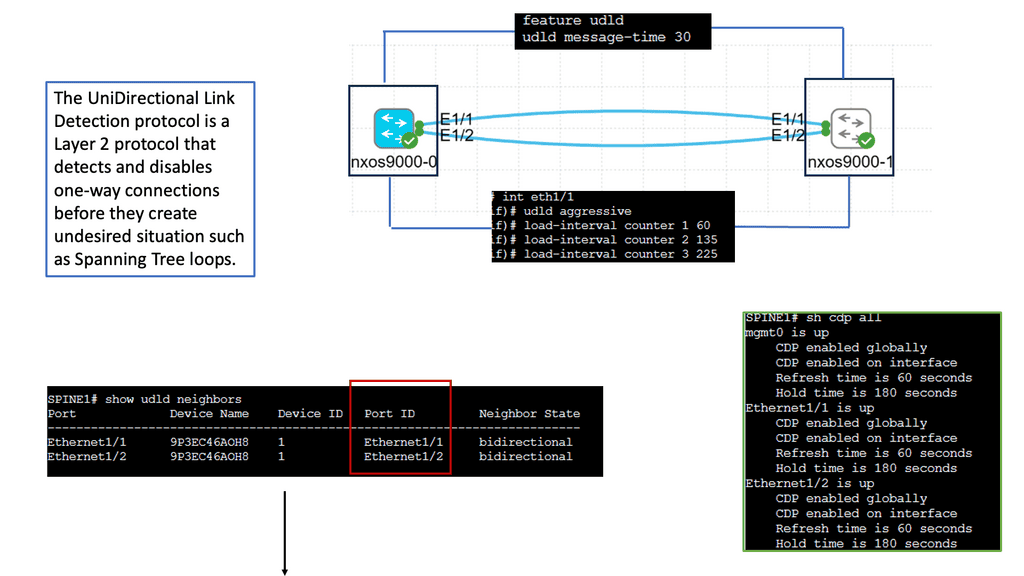
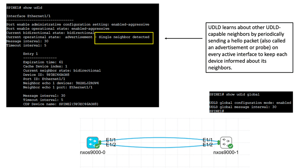
UDLD, at its core, is a layer 2 protocol designed to detect and mitigate unidirectional links in Ethernet connections. It actively monitors the link status, allowing network devices to promptly detect and address potential issues. By verifying the bidirectional communication between neighboring devices, UDLD acts as a guardian, preventing one-way communication breakdowns.
Implementing UDLD brings forth numerous advantages for network administrators and organizations alike.
Firstly, it enhances network reliability by identifying and resolving unidirectional link failures that could otherwise lead to data loss and network disruptions.
Secondly, UDLD helps troubleshoot by providing valuable insights into link quality and integrity. This proactive approach aids in reducing downtime and improving overall network performance.
Enhancing Routing Convergence
Network administrators can implement various strategies to improve routing convergence. One approach is to utilize route summarization, which reduces the number of routes advertised and processed by routers. This helps minimize the impact of changes in specific network segments on overall convergence time.
Furthermore, implementing fast link failure detection mechanisms, such as Bidirectional Forwarding Detection (BFD), can significantly reduce convergence time. BFD allows routers to quickly detect link failures and trigger immediate updates to routing tables, ensuring faster convergence.
**Factors Influencing Routing Convergence**
Several factors impact routing convergence in a network. Firstly, the efficiency of the routing protocols being used plays a crucial role. Protocols such as OSPF (Open Shortest Path First) and EIGRP (Enhanced Interior Gateway Routing Protocol) are designed to facilitate fast convergence by quickly adapting to network changes.
Additionally, network topology and scale can affect routing convergence. Large networks with complex topologies may require more time for routers to converge due to the increased number of routes and potential link failures. Network administrators must carefully design and optimize the network architecture to minimize convergence time.
Control and data plane
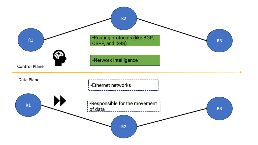
When considering routing convergence with forwarding routing protocols, we must first highlight that a networking device is tasked with two planes of operation—the control plane and the data plane. The job of the data plane is to switch traffic across the router’s interfaces as fast as possible, i.e., move packets. The control plane has the more complex operation of putting together and creating the controls so the data plane can operate efficiently. How these two planes interact will affect network convergence time.
The network’s control plane finds the best path for routing convergence from any source to any network destination. For quick convergence routing, it must react quickly and dynamically to changes in the network, both on the LAN and on the WAN.
Monitoring and Troubleshooting Routing Convergence
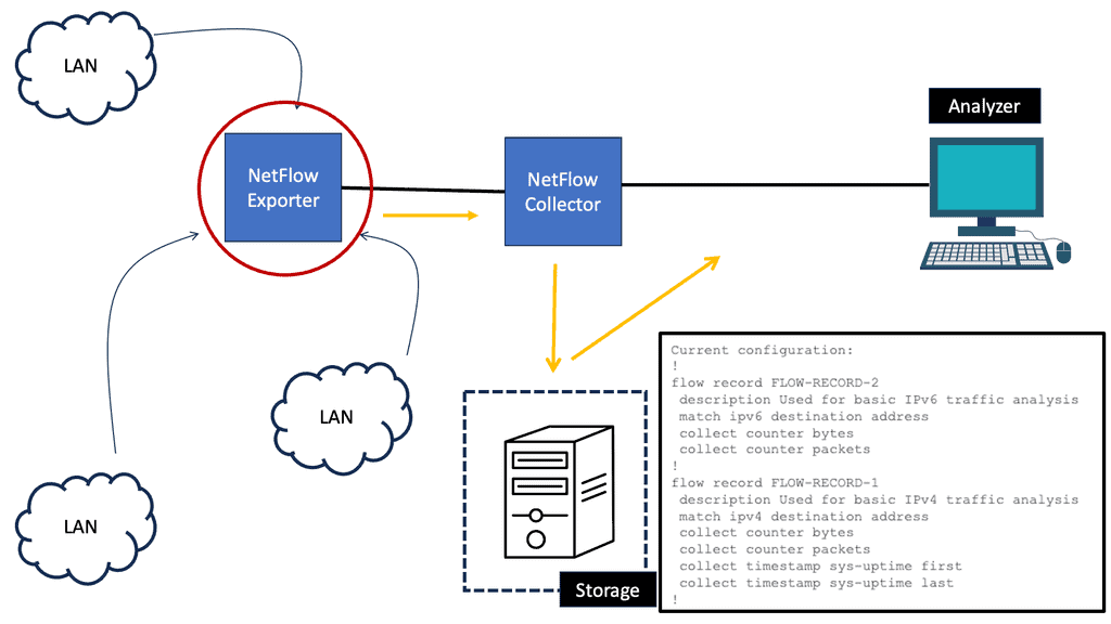
Network administrators must monitor routing convergence to identify and promptly address potential issues. Network management tools, such as SNMP (Simple Network Management Protocol) and NetFlow analysis, can provide valuable insights into routing convergence performance, including convergence time, route flapping, and stability.
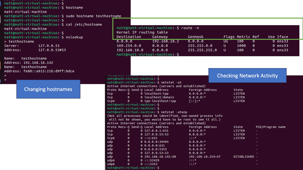
When troubleshooting routing convergence problems, administrators should carefully analyze routing table updates, link state information, and routing protocol logs. This information can help pinpoint the root cause of convergence delays or inconsistencies, allowing for targeted remediation.
Related: For pre-information, you may find the following posts helpful:
Convergence Time Definition.
I found two similar definitions of convergence time:
“Convergence is the amount of time ( and thus packet loss ) after a failure in the network and before the network settles into a steady state.” Also, ” Convergence is the amount of time ( and thus packet loss) after a failure in the network and before the network responds to the failure.”
The difference between the two convergence time definitions is subtle but essential – steady-state vs. just responding. The control plane and its reaction to topology changes can be separated into four parts below. Each area must be addressed individually, as leaving one area out results in slow network convergence time and application time-out.
**IP routing**
Moving IP Packets
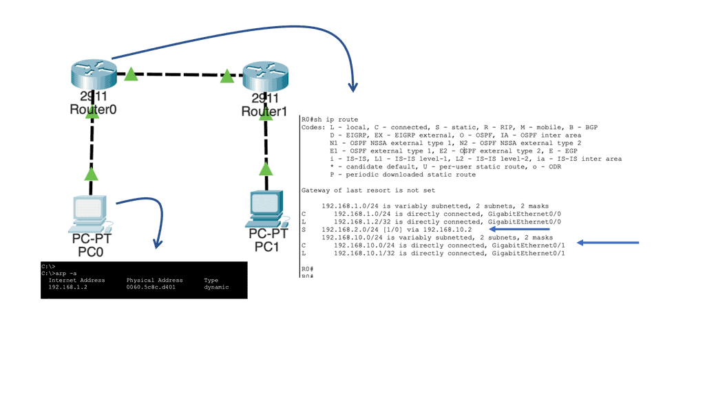
A router’s primary role is moving an IP packet from one network to another. Routers select the best loop-free path in a network to forward a packet to its destination IP address. A router learns about nonattached networks through static configuration or dynamic IP routing protocols. Both static and dynamic are examples of routing protocols.
With dynamic IP routing protocols, we can handle network topology changes dynamically. Here, we can distribute network topology information between routers in the network. When there is a change in the network topology, the dynamic routing protocol provides updates without intervention when a topology change occurs.
On the other hand, we have IP routing to static routes, which do not accommodate topology changes very well and can be a burden depending on the network size. However, static routing is a viable solution for minimal networks with no modifications.
Knowledge Check: Bidirectional Forwarding Detection
Understanding BFD
BFD is a lightweight protocol designed to detect faults in the forwarding path between network devices. It operates at a low level, constantly monitoring the connectivity and responsiveness of neighboring devices. BFD can quickly detect failures by exchanging control packets and taking appropriate action to maintain network stability.
The Benefits of BFD
The implementation of BFD brings numerous advantages to network administrators and operators. Firstly, it provides rapid fault detection, reducing downtime and minimizing the impact of network failures. Additionally, BFD offers scalable and efficient operation, as it consumes minimal network resources. This makes it an ideal choice for large-scale networks where resource optimization is crucial.
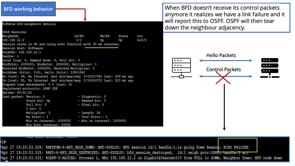
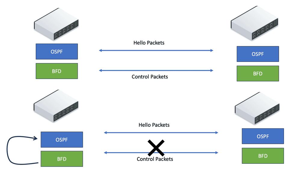
BFD runs independently from other (routing) protocols. Once it’s up and running, you can configure protocols like OSPF, EIGRP, BGP, HSRP, MPLS LDP, etc., to use BFD for link failure detection instead of their mechanisms. When the link fails, BFD informs the protocol. When BFD no longer receives its control packets, it realizes we have a link failure and reports this to OSPF. OSPF will then tear down the neighbor adjacency.
Use Cases of BFD
BFD finds its applications in various networking scenarios. One prominent use case is link aggregation, where BFD helps detect link failures and ensures seamless failover to alternate links. BFD is also widely utilized in Virtual Private Networks (VPNs) to monitor the connectivity of tunnel endpoints, enabling quick detection of connectivity issues and swift rerouting.
Implementing BFD in Practice
Implementing BFD requires careful consideration and configuration. Network devices must be appropriately configured to enable BFD sessions and define appropriate parameters such as timers and thresholds. Additionally, network administrators must ensure proper integration with underlying routing protocols to maximize BFD’s efficiency.
Convergence Routing and Network Convergence Time
Network convergence connects multiple computer systems, networks, or components to establish communication and efficient data transfer. However, it can be a slow process, depending on the size and complexity of the network, the amount of data that needs to be transferred, and the speed of the underlying technologies.
For networks to converge, all of the components must interact with each other and establish rules for data transfer. This process requires that the various components communicate with each other and usually involves exchanging configuration data to ensure that all components use the same protocols.
Network convergence is also dependent on the speed of the underlying technologies.
To speed up convergence, administrators should use the latest technologies, minimize the amount of data that needs to be transferred, and ensure that all components are correctly configured to be compatible. By following these steps, network convergence can be made faster and more efficient.
Example: OSPF
To put it simply, convergence or routing convergence is a state in which a set of routers in a network share the same topological information. For example, we have ten routers in one OSFP area. OSPF is an example of a fast-converging routing protocol. A network of a few OSPF routers can converge in seconds.
The routers within the OSPF area in the network collect the topology information from one another through the routing protocol. Depending on the routing protocol used to collect the data, the routers in the same network should have identical copies of routing information.
Different routing protocols will have additional convergence time. The time the routers take to reach convergence after a change in topology is termed convergence time. Fast network convergence and fast failover are critical factors in network performance. Before we get into the details of routing convergence, let us recap how networking works.
Unlike IS-IS, OSPF has fewer “knobs” for optimizing convergence. This is probably because IS-IS is being developed and supported by a separate team geared towards ISPs, where fast convergence is a competitive advantage.
OSPF: Incremental SPF
OSPF calculates the SPT (Shortest Path Tree) using the SPF (Shortest Path First) algorithm. SPTs are built by OSPF routers within the same area with the same LSAs, LSDBs, and LSAs. OSPF routers will rerun a full SPF calculation even when there is just a single change in the network topology (change to an LSA type 1 and LSA type 2).
If a topology change occurs, we should run a full SPT calculation to find the shortest paths to all destinations. Unfortunately, we also calculate paths that have not changed since the last SPF.
In incremental SPF, OSPF only recalculates the parts of the SPT that have changed.
Because you don’t run a full SPF all the time, the router’s CPU load decreases,, and convergence times improve—additionally, your router stores the previous SPT copy, which requires more memory.
In three scenarios, incremental SPF is beneficial:
Adding (or removing) a leaf node to a branch
Link failure in non-SPT
Link failure in a branch of SPT
When many routers are in a single area, and the CPU load is high because of OSPF, incremental SPF can be enabled per router.
Forwarding Paradigms
We have bridging routing and switching with data and the control plane. So, we need to get packets across a network, which is easy if we have a single cable. You need to find the node’s address, and small and non-IP protocols would use a broadcast. When devices in the middle break this path, we can use source routing, path-based forwarding, and hop-by-hop address-based forwarding based solely on the destination address.
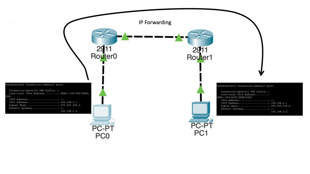
When protocols like IP came into play, hop-by-hop destination-based forwarding became the most popular; this is how IP forwarding works. Everyone in the path makes independent forwarding decisions. Each device looks at the destination address, examines its lookup tables, and decides where to send the packet.
**Finding paths across the network**
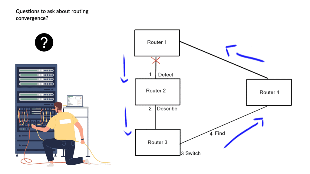
How do we find a path across the network? We know there are three ways to get packets across the network – source routing, path-based forwarding, and hop-by-hop destination-based forwarding. So, we need some way to populate the forwarding tables. You need to know how your neighbors are and who your endpoints are. This can be static routing, but it is more likely to be a routing protocol. Routing protocols have to solve and describe the routing convergence on the network at a high level.
When we are up and running, events can happen to the topology that force or make the routing protocols react and perform a convergence routing state. For example, we have a link failure, and the topology has changed, impacting our forwarding information. So, we must propagate the information and adjust the path information after the topology change. We know these convergence routing states are to detect, describe, switch, and find.
Rouitng Convergence | Convergence |
To better understand routing convergence, I would like to share the network convergence time for each routing protocol before diving into each step. The times displayed below are from a Cisco Live session based on real-world case studies and field research. We are separating each of the convergence routing steps described above into the following fields: Detect, describe, find alternative, and total time.
Routing Protocol | RIP | OSPF | EIGRP |
Detect | <1 second-best, 105 seconds average | <1 second-best, 20 seconds average | <1 second-best, 15 seconds average.30 seconds worst |
Describe | 15 seconds average, 30 seconds worst | 1 second-best, 5 seconds average. | 2 seconds |
Find Alternative | 15 seconds average, 30 seconds worst | 1-second average. | *** <500ms per query hop average Assume a 2-second average |
Total Time | Best Average Case: 31 seconds Average Case: 135 seconds Worse Case: 179 seconds | Best Average Case: 2 to 3 seconds Average Case: 25 seconds Worse Case: 45 seconds | Best Average Case: <1 second Average Case: 20 seconds Worse Case: 35 seconds |
*** The alternate route is found before the described phase due to the feasible successor design with EIGRP path selection.
Convergence Routing
Convergence routing: EIGPR
EIGRP is the fastest but only fractional. EIGRP has a pre-built loop-free path known as a feasible successor. The FS route has a higher metric than the successor, making it a backup route to the successor route. The effect of a pre-computed backup route on convergence is that EIGRP can react locally to a change in the network topology; nowadays, this is usually done in the FIB. EIGRP would have to query for the alternative route without a feasible successor, increasing convergence time.
However, you can have a Loop Free Alternative ( LFA ) for OSPF, which can have a pre-computed alternate path. Still, LFAs can only work with specific typologies and don’t guarantee against micro-loops ( EIGRP guarantees against micro-loops).
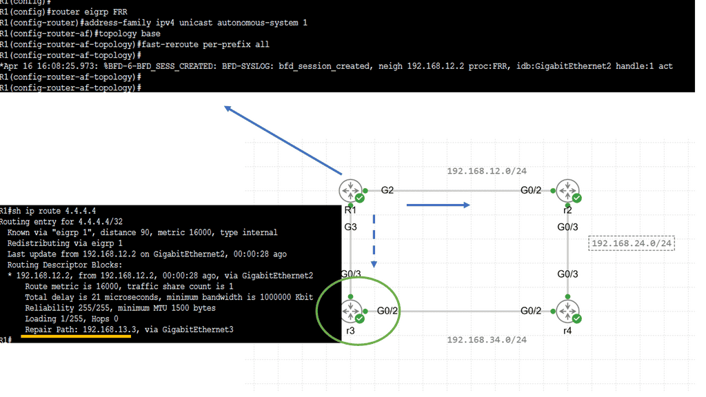
Lab Guide: EIGRP LFA FRR
With Loop-Free Alternate (LFA) Fast Reroute (FRR), EIGRP can switch to a backup path in less than 50 milliseconds. Fast rerouting means switching to another next hop, and a loop-free alternate refers to a loop-free alternative path.
Perhaps this sounds familiar to you. After all, EIGRP has feasible successors. The alternate paths calculated by EIGRP are loop-free. As soon as the successor fails, EIGRP can use a feasible successor.
It’s true, but there’s one big catch. In the routing table, EIGRP feasible successors are not immediately installed. Only one route is installed, the successor route. EIGRP installs the feasible successor when the successor fails, which takes time. By installing both successor routes and feasible successor routes in the routing table, fast rerouting makes convergence even faster.
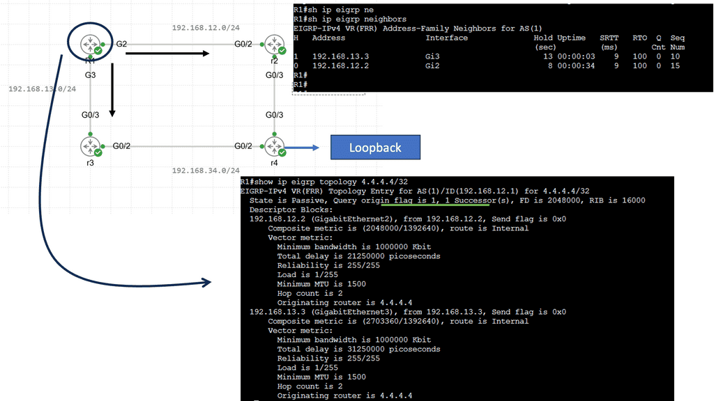
These four routers run EIGRP; there’s a loopback on R4 with network 4.4.4.4/32. R1 can go through R2 or R3 to get there. The delay on R1’s GigabitEthernet3 interface has increased, so R2 is our successor, and R3 is our feasible successor. The output below is interesting. We still see the successor route, but at the bottom, you can see the repair path…that’s our feasible successor.
TCP Congestion control
Ask yourself, is < 1-second convergence fast enough for today’s applications? Indeed, the answer would be yes for some non-critical applications that work on TCP. TCP has built-in backoff algorithms that can deal with packet loss by re-transmitting to recover lost segments. However, non-bulk data applications like video and VOIP have stricter rules and require fast convergence and minimal packet loss.
For example, a 5-second delay in routing protocol convergence could mean several hundred dropped voice calls. A 50-second delay in a Gigabit Ethernet link implies about 6.25 GB of lost information.
Adding Resilience
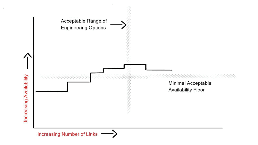
To add resilience to a network, you can aim to make the network redundant. When you add redundancy, you are betting that outages of the original path and the backup path will not co-occur and that the primary path does not fate share with the backup path ( they do not share common underlying infrastructure, i.e., physical conducts or power ).
There needs to be a limit on the number of links you add to make your network redundant, and adding 50 extra links does not make your network 50 times more redundant. It does the opposite! The control plane is tasked with finding the best path and must react to modifications in the network as quickly as possible.
However, every additional link you add slows down the convergence of the router’s control plane as there is additional information to compute, resulting in longer convergence times. The correct number of backup links is a trade-off between redundancy versus availability. The optimal level of redundancy between two points should be two or three links. The fourth link would make the network converge slower.
Routing Convergence and Routing Protocol Algorithms
Routing protocol algorithms can be tweaked to exponentially back off and deal with bulk information. However, no matter how many timers you use, the more data in the routing databases, the longer the convergence times. The primary way to reduce network convergence is to reduce the size of your routing tables by accepting just a default route, creating a flooding boundary domain, or using some other configuration method.
For example, a common approach in OSPF to reduce the size of routing tables and flooding boundaries is to create OSPF stub areas. OSPF stub areas limit the amount of information in the area. For example, EIGRP limits the flooding query domain by creating EIGRP stub routers and intelligently designing aggregation points. Now let us revisit the components of routing convergence:
Routing Convergence Step | Routing Convergence Details |
Step 1 | Failure detection |
Step 2 | Failure propagation ( flooding, etc.) IGP Reaction |
Step 3 | Topology/Routing calculation. IGP Reaction. |
Step 4 | Update the routing and forwarding table ( RIB & FIB) |
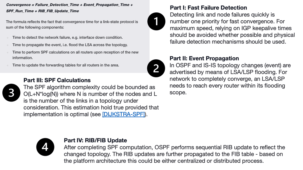
**Stage 1: Failure Detection**
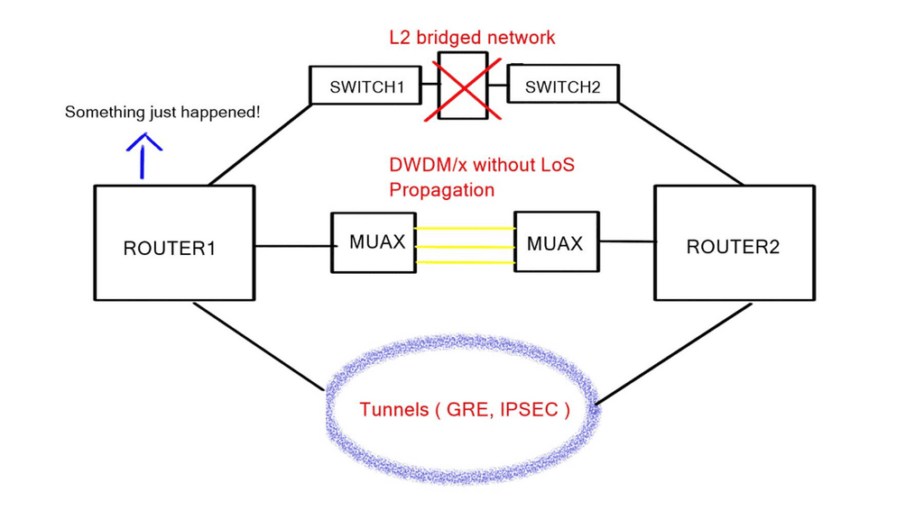
The first and foremost problem facing the control plane is quickly detecting topology changes. Detecting the failure is the most critical and challenging part of network convergence. It can occur at different layers of the OSI stack – Physical Layers ( Layer 1), Data Link Layer ( Layer 2 ), Network Layer ( Layer 3 ), and Application layer ( Layer 7 ). There are many types of techniques used to detect link failures, but they all generally come down to two basic types:
- Event-driven notification occurs when a carrier is lost or when one network element detects a failure and notifies the other network elements.
- Polling-driven notification – generally HELLO protocols that test the path for reachability, such as Bidirectional Forwarding Detection ( BFD ). Event-driven notifications are always preferred over polling-driven ones as the latter have to wait for three polls before declaring a path down. However, there are some cases when you have multiple Layer devices in the path, and HELLO polling systems are the only method that can be used to detect a failure.
Layer 1 failure detection
Layer 1: Ethernet mechanisms like auto-negotiation ( 1 GigE ) and link fault signaling ( 10 GigE 802.3ae/ 40 GigE 802.3ba ) can signal local failures to the remote end.
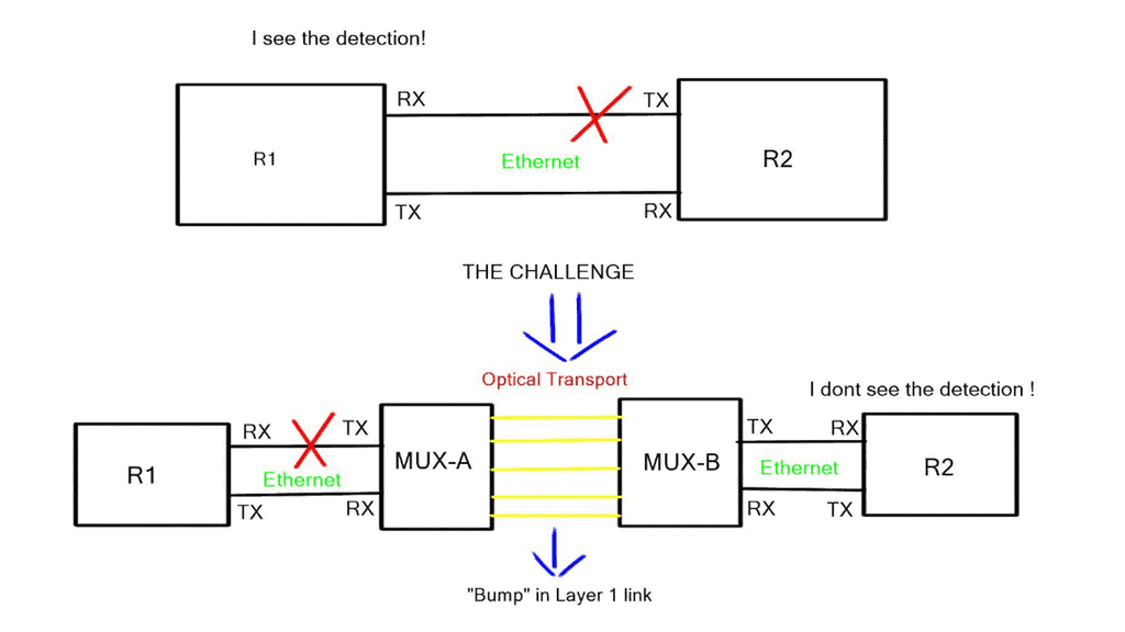
However, the challenge is getting the signal across an optical cloud, as relaying the fault information to the other end is impossible. When there is a “bump” in the Layer 1 link, it is not always possible for the remote end to detect the failure. In this case, the link fault signaling from Ethernet would get lost in the service provider’s network.
The actual link-down / interface-down event detection is hardware-dependent. Older platforms, such as the 6704 line cards for the Catalyst 6500, used a per-port polling mechanism, resulting in a 1 sec detect link failure period. More recent Nexus switches and the latest Catalyst 5600 line cards have an interrupt-driven notification mechanism resulting in high-speed and predictable link failure detection.
Layer 2 failure detection
Layer 2: The layer 2 detection mechanism will kick in if the Layer 1 mechanism does not. Unidirectional Link Detection ( UDLD ) is a Cisco proprietary lightweight Layer 2 failure detection protocol designed for detecting one-way connections due to physical or soft failure and miss-wirings.
- A key point: UDLD is a slow protocol
UDLD is a reasonably slow protocol that uses an average of 15 seconds for message interval and 21 seconds for detection. Its period has raised questions about its use in today’s data centers. However, the chances of miswirings are minimal; Layer 1 mechanisms always communicate unidirectional physical failure, and STP Bridge Assurance takes care of soft failures in either direction.
STP Bridge assurance turns STP into a bidirectional protocol and ensures that the spanning tree never fails to open and only fails to close. Failing open means that if a switch does not hear from its neighbor, it immediately starts forwarding on initially blocked ports, causing network havoc.
Layer 3 failure detection
Layer 3: In some cases, failure detection has to reply to HELLO protocols at Layer 3. This is needed when there are intermediate Layer 2 hops over Layer links and concerns over uni-direction failures on point-to-point physical links arise.
All Layer 3 protocols use HELLOs to maintain neighbor adjacency and a DEAD time to declare a neighbor dead. These timers can be tuned for faster convergence. However, it is generally not recommended due to the increase in CPU utilization causing false positives and the challenges ISSU and SSO face. They enable bidirectional forwarding detection ( BFD ) as the layer 3 detection mechanism is strongly recommended over aggressive protocol times, and they use BFD for all protocols.
Bidirectional Forwarding Detection ( BFD ) is a lightweight hello protocol for sub-second Layer 3 failure detection. It can run over multiple transport protocols, such as MPLS, THRILL, IPv6, and IPv4, making it the preferred method.
**Stage 2: Routing convergence and failure propagation**
When a change occurs in the network topology, it must be registered with the local router and transmitted throughout the rest of the network. The transmission of the change information will be carried out differently for Link-State and Distance Vector protocols. Link state protocols must flood information to every device in the network, and the distance vector must process the topology change at every hop through the network.
The processing of information at every hop may lead you to conclude that link-state protocols always converge more quickly than path-vector protocols, but this is not the case. EIGRP, due to its pre-computed backup path, will converge more rapidly than any link-state protocol.
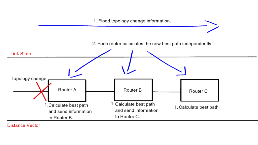
To propagate topology changes as quickly as possible, OSPF ( Link state ) can group changes into a few LSA while slowing down the rate at which information is flooded, i.e., do not flood on every change. This is accomplished with link-state flood timer tuning combined with exponential backoff systems, such as link-state advertisement delay / initial link-state advertisement throttle delay.
Unfortunately, Distance Vector Protocols do not have such timers. Therefore, reducing the routing table size is the only option for EIGRP. This can be done by aggregating and filtering reachability information ( summary route or Stub areas ).
**Stage 3: Topology/Routing calculation**
Similar to the second step, link-state protocols use exponential back-off timers in this step. These timers adjust the waiting time for OSPF and ISIS to wait after receiving new topology information before calculating the best path.
**Stage 4: Update the routing and forwarding table ( RIB & FIB)**
Finally, after the topology information has been flooding through the network and a new best path has been calculated, the new best path must be installed in the Forwarding Information Base ( FIB ). The FIB is a copy of the RIB in hardware, and the forwarding process finds it much easier to read than the RIB. However, again, this is usually done in hardware. Most vendors offer features that will install a pre-computed backup path on the line cards forwarding table so the fail-over from the primary path to the backup path can be done milliseconds without interrupting the router CPU.
Closing Points: Routing Convergence
Routing convergence refers to the process by which network routers exchange routing information and adapt to changes in network topology or routing policies. It involves the timely update and synchronization of routing tables across the network, allowing routers to determine the best paths for forwarding data packets.
Routing convergence is vital for maintaining network stability and minimizing disruptions. Network traffic may experience delays, bottlenecks, or even failures without proper convergence. Routing convergence enables efficient and reliable communication by ensuring all network routers have consistent routing information.

- DMVPN - May 20, 2023
- Computer Networking: Building a Strong Foundation for Success - April 7, 2023
- eBOOK – SASE Capabilities - April 6, 2023