### Types of Load Balancers
Load balancers come in various forms, each designed to suit different needs and environments. Primarily, they are categorized as hardware, software, and cloud-based load balancers. Hardware load balancers are physical devices, offering high performance but at a higher cost. Software load balancers are more flexible and cost-effective, running on standard servers. Lastly, cloud-based load balancers are gaining popularity due to their scalability and ease of integration with modern cloud environments.
### How Load Balancing Works
The process of load balancing involves several sophisticated algorithms. Some of the most common ones include Round Robin, where requests are distributed sequentially, and Least Connections, which directs traffic to the server with the fewest active connections. More advanced algorithms might take into account server response times and geographical locations to optimize performance further.
GTM load balancing is a technique used to distribute network or application traffic efficiently across multiple global servers. This ensures not only optimal performance but also increased reliability and availability for users around the globe. In this blog post, we’ll delve into the intricacies of GTM load balancing and explore how it can benefit your organization.
### How GTM Load Balancing Works
At its core, GTM load balancing involves directing user requests to the most appropriate server based on a variety of criteria, such as geographical location, server load, and network conditions. This is achieved through DNS-based routing, where the GTM system evaluates the best server to handle a request. By intelligently directing traffic, GTM load balancing minimizes latency, reduces server load, and enhances the user experience. Moreover, it provides a robust mechanism for disaster recovery by rerouting traffic to alternative servers in case of a failure.
Understanding GTM Load Balancer
A GTM load balancer is a powerful networking tool that intelligently distributes incoming traffic across multiple servers. It acts as a central management point, ensuring that each request is efficiently routed to the most appropriate server. Whether for a website, application, or any online service, a GTM load balancer is crucial in optimizing performance and ensuring high availability.
-Enhanced Scalability: A GTM load balancer allows businesses to scale their infrastructure seamlessly by evenly distributing traffic. As the demand increases, additional servers can be added without impacting the end-user experience. This scalability helps businesses handle sudden traffic spikes and effectively manage growth.
-Improved Performance: With a GTM load balancer in place, the workload is distributed evenly, preventing any single server from overloading. This results in improved response times, reduced latency, and enhanced user experience. By intelligently routing traffic based on factors like server health, location, and network conditions, a GTM load balancer ensures that each user request is directed to the best-performing server.
High Availability and Failover
-Redundancy and Failover Protection: A key feature of a GTM load balancer is its ability to ensure high availability. By constantly monitoring the health of servers, it can detect failures and automatically redirect traffic to healthy servers. This failover mechanism minimizes service disruptions and ensures business continuity.
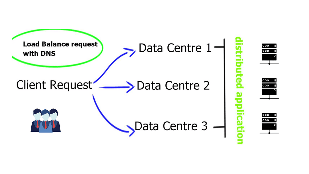
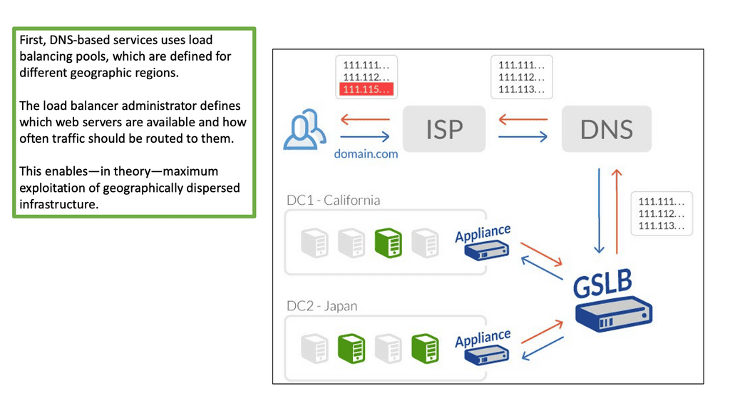
-Global Server Load Balancing (GSLB): A GTM load balancer offers GSLB capabilities for businesses with a distributed infrastructure across multiple data centers. It can intelligently route traffic to the most suitable data center based on server response time, network congestion, and user proximity.
Flexibility and Traffic Management
– Geographic Load Balancing: A GTM load balancer can route traffic based on the user’s geographic location. By directing requests to the nearest server, businesses can minimize latency and deliver a seamless experience to users across different regions.
– Load Balancing Algorithms: GTM load balancers offer various load-balancing algorithms to cater to different needs. Businesses can choose the algorithm that suits their requirements, from simple round-robin to more advanced algorithms like weighted round-robin, least connections, and IP hash.
Example: Load Balancing with HAProxy
Understanding HAProxy
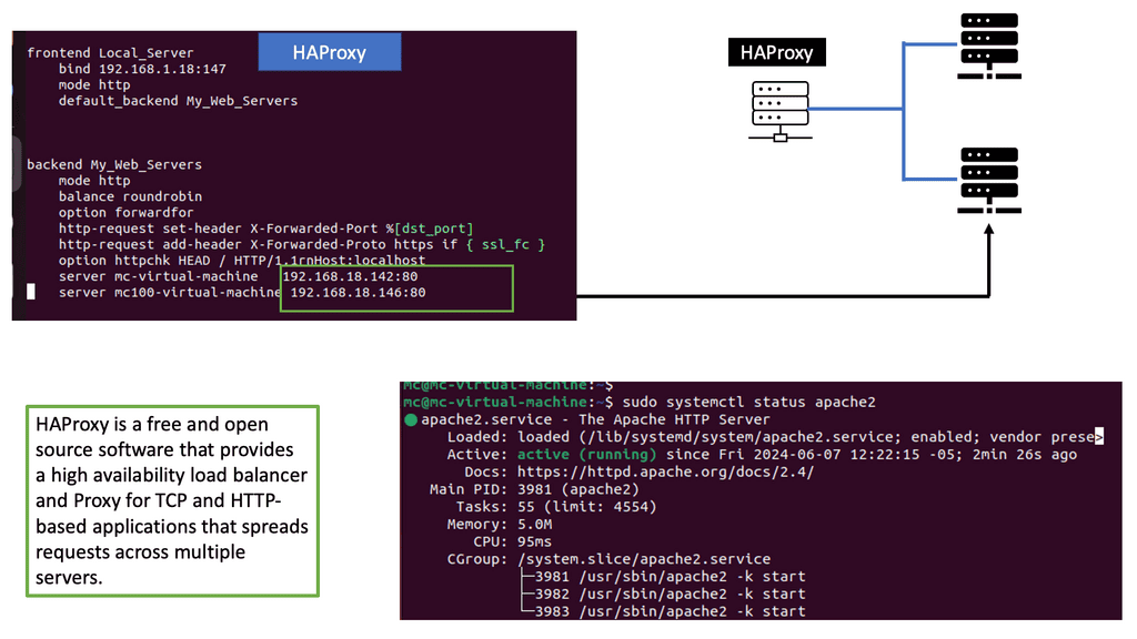
HAProxy, an open-source software, acts as a load balancer and proxy server. Its primary function is to distribute incoming web traffic across multiple servers, ensuring optimal utilization of resources. With its robust set of features and flexibility, HAProxy has become a go-to solution for high-performance web architectures.
HAProxy offers a plethora of features that empower businesses to achieve high availability and scalability. Some notable features include:
1. Load Balancing: HAProxy intelligently distributes incoming traffic across backend servers, preventing overloading and ensuring even resource utilization.
2. SSL/TLS Offloading: By offloading SSL/TLS encryption to HAProxy, backend servers are relieved from the computational overhead, resulting in improved performance.
3. Health Checking: HAProxy continuously monitors the health of backend servers, automatically routing traffic away from unresponsive or faulty servers.
4. Session Persistence: It provides session stickiness, allowing users to maintain their session state even when requests are served by different servers.
Key Features of GTM Load Balancer:
1. Geographic Load Balancing: GTM Load Balancer uses geolocation-based routing to direct users to the nearest server location. This reduces latency and ensures that users are connected to the server with the lowest network hops, resulting in faster response times.
2. Health Monitoring: The load balancer continuously monitors the health and availability of servers. If a server becomes unresponsive or experiences a high load, GTM Load Balancer automatically redirects traffic to healthy servers, minimizing service disruptions and maintaining high availability.
3. Flexible Load Balancing Algorithms: GTM Load Balancer offers a range of load balancing algorithms, including round-robin, weighted round-robin, and least connections. These algorithms enable businesses to customize the traffic distribution strategy based on their specific needs, ensuring optimal performance for different types of web applications.
Knowledge Check: TCP Performance Parameters
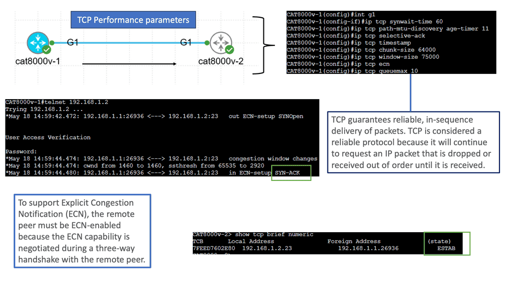
TCP (Transmission Control Protocol) is a fundamental protocol that enables reliable communication over the Internet. Understanding and fine-tuning TCP performance parameters are crucial to ensuring optimal performance and efficiency. In this blog post, we will explore the key parameters impacting TCP performance and how they can be optimized to enhance network communication.
TCP Window Size: The TCP window size represents the amount of data that can be sent before receiving an acknowledgment. It plays a pivotal role in determining the throughput of a TCP connection. Adjusting the window size based on network conditions, such as latency and bandwidth, can optimize TCP performance.
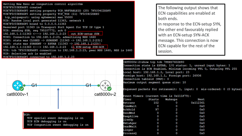
TCP Congestion Window: Congestion control algorithms regulate data transmission rate to avoid network congestion. The TCP congestion window determines the maximum number of unacknowledged packets in transit at any given time. Understanding different congestion control algorithms, such as Reno, New Reno, and Cubic, helps select the most suitable algorithm for specific network scenarios.
Duplicate ACKs and Fast Retransmit: TCP utilizes duplicate ACKs (Acknowledgments) to identify packet loss. Fast Retransmit triggers the retransmission of a lost packet upon receiving a certain number of duplicate ACKs. By adjusting the parameters related to Fast Retransmit and Recovery, TCP performance can be optimized for faster error recovery.
Nagle’s Algorithm: Nagle’s Algorithm aims to optimize TCP performance by reducing the number of small packets sent across the network. It achieves this by buffering small amounts of data before sending, thus reducing the overhead caused by frequent small packets. Additionally, adjusting the Delayed Acknowledgment timer can improve TCP efficiency by reducing the number of ACK packets sent.
The Role of Load Balancing
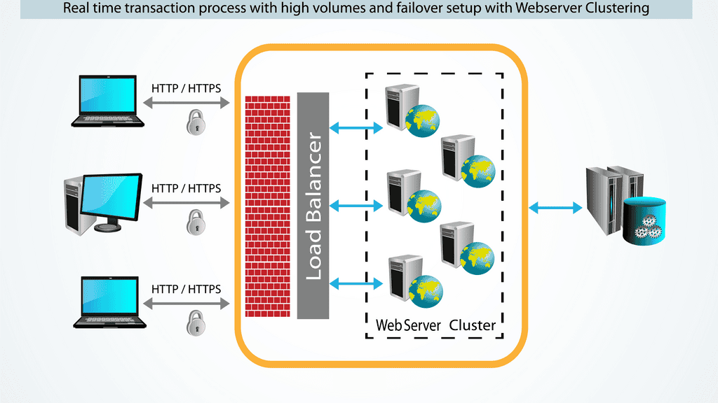
Load balancing involves spreading an application’s processing load over several different systems to improve overall performance in processing incoming requests. It splits the load that arrives into one server among several other devices, which can decrease the amount of processing done by the primary receiving server.
While splitting up different applications used to process a request among separate servers is usually the first step, there are several additional ways to increase your ability to split up and process loads—all for greater efficiency and performance. DNS load balancing failover, which we will discuss next, is the most straightforward way to load balance.
DNS Load Balancing
DNS load balancing is the simplest form of load balancing. However, it is also one of the most powerful tools available. Directing incoming traffic to a set of servers quickly solves many performance problems. In spite of its ease and quickness, DNS load balancing cannot handle all situations.
A DNS server is a cluster of servers that answer queries together but cannot handle every DNS query on the planet. The solution lies in caching. Your system looks up servers from its storage by keeping a list of known servers in a cache. As a result, you can reduce the time it takes to walk a previously visited server’s DNS tree. Furthermore, it reduces the number of queries sent to the primary nodes.
The Role of a GTM Load Balancer
A GTM Load Balancer is a solution that efficiently distributes traffic across multiple web applications and services. In addition, it distributes traffic across various nodes, allowing for high availability and scalability. As a result, these load balancers enable organizations to improve website performance, reduce costs associated with hardware, and allow seamless scaling as application demand increases. It acts as a virtual traffic cop, ensuring incoming requests are routed to the most appropriate server or data center based on predefined rules and algorithms.
A Key Point: LTM Load Balancer
The LTM Load Balancer, short for Local Traffic Manager Load Balancer, is a software-based solution that distributes incoming requests across multiple servers. This ensures efficient resource utilization and prevents any single server from being overwhelmed. By intelligently distributing traffic, the LTM Load Balancer ensures high availability, scalability, and improved performance for applications and services.
GTM Load Balancing:
Continuously Monitors:
GTM Load Balancers continuously monitor server health, network conditions, and application performance. They use this information to distribute incoming traffic intelligently, ensuring that each server or data center operates optimally. By spreading the load across multiple servers, GTM Load Balancers prevent any single server from becoming overwhelmed, thus minimizing the risk of downtime or performance degradation.
Traffic Patterns:
GTM Load Balancers are designed to handle a variety of traffic patterns, such as round robin, least connections, and weighted least connections. It can also be configured to use dynamic server selection, allowing for high flexibility and scalability. GTM Load Balancers work with HTTP, HTTPS, TCP, and UDP protocols, which are well-suited to handle various applications and services.
GTM Load Balancers can be deployed in public, private, and hybrid cloud environments, making them a flexible and cost-effective solution for businesses of all sizes. They also have advanced features such as automatic failover, health checks, and SSL acceleration.
**Benefits of GTM Load Balancer**
1. Enhanced Website Performance: By efficiently distributing traffic, GTM Load Balancer helps balance the server load, preventing any single server from being overwhelmed. This leads to improved website performance, faster response times, and reduced latency, resulting in a seamless user experience.
2. Increased Scalability: As online businesses grow, the demand for server resources increases. GTM Load Balancer allows enterprises to scale their infrastructure by adding more servers or data centers. This ensures that the website can handle increasing traffic without compromising performance.
3. Improved Availability and Redundancy: GTM Load Balancer offers high availability by continuously monitoring server health and automatically redirecting traffic away from any server experiencing issues. It can detect server failures and quickly reroute traffic to healthy servers, minimizing downtime and ensuring uninterrupted service.
4. Geolocation-based Routing: Businesses often cater to a diverse audience across different regions in a globalized world. GTM Load Balancer can intelligently route traffic based on the user’s geolocation, directing them to the nearest server or data center. This reduces latency and improves the overall user experience.
5. Traffic Steering: GTM Load Balancer allows businesses to prioritize traffic based on specific criteria. For example, it can direct high-priority traffic to servers with more resources or specific geographic locations. This ensures that critical requests are processed efficiently, meeting the needs of different user segments.
Knowledge Check: Understanding TCP MSS
TCP MSS refers to the maximum amount of data encapsulated within a single TCP segment. It plays a crucial role in determining the efficiency and reliability of data transmission over TCP connections. By restricting the segment size, TCP MSS ensures that data can be transmitted without fragmentation, optimizing network performance.
Several factors come into play when determining the appropriate TCP MSS for a given network environment. One key factor is the underlying network layer’s Maximum Transmission Unit (MTU). The MTU defines the maximum size of packets that can be transmitted over the network. TCP MSS needs to be set lower than the MTU to avoid fragmentation. Network devices such as firewalls and routers may also impact the effective TCP MSS.
Configuring TCP MSS involves making adjustments at both ends of the TCP connection. It is typically done by setting the MSS value within the TCP headers. On the server side, the MSS value can be adjusted in the operating system’s TCP stack settings. Similarly, on the client side, applications or operating systems may provide ways to modify the MSS value. Careful consideration and testing are necessary to find the optimal TCP MSS for a network infrastructure.
The choice of TCP MSS can significantly impact network performance. Setting it too high may lead to increased packet fragmentation and retransmissions, causing delays and reducing overall throughput. Conversely, setting it too low may result in inefficient bandwidth utilization. Finding the right balance is crucial to ensuring smooth and efficient data transmission.

Related: Both of you proceed. You may find the following helpful information:
- DNS Security Solutions
- OpenShift SDN
- ASA Failover
- Load Balancing and Scalability
- Data Center Failover
- Application Delivery Architecture
- Port 179
- Full Proxy
- Load Balancing
GTM load balancer
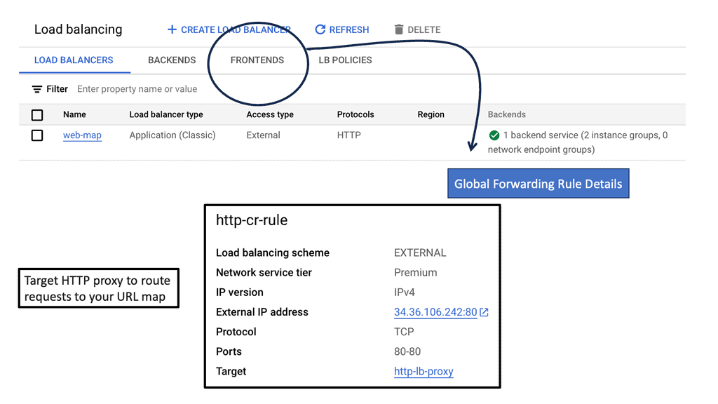
A load balancer is a specialized device or software that distributes incoming network traffic across multiple servers or resources. Its primary objective is evenly distributing the workload, optimizing resource utilization, and minimizing response time. By intelligently routing traffic, load balancers prevent any single server from being overwhelmed, ensuring high availability and fault tolerance.
Load Balancer Functions and Features
Load balancers offer many functions and features that enhance network performance and scalability. Some essential functions include:
1. Traffic Distribution: Load balancers efficiently distribute incoming network traffic across multiple servers, ensuring no single server is overwhelmed.
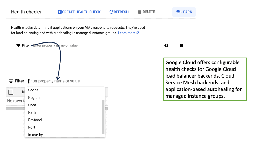
2. Health Monitoring: Load balancers continuously monitor the health and availability of servers, automatically detecting and avoiding faulty or unresponsive ones.
3. Session Persistence: Load balancers can maintain session persistence, ensuring that requests from the same client are consistently routed to the same server, which is essential for specific applications.
4. SSL Offloading: Load balancers can offload the SSL/TLS encryption and decryption process, relieving the backend servers from this computationally intensive task.
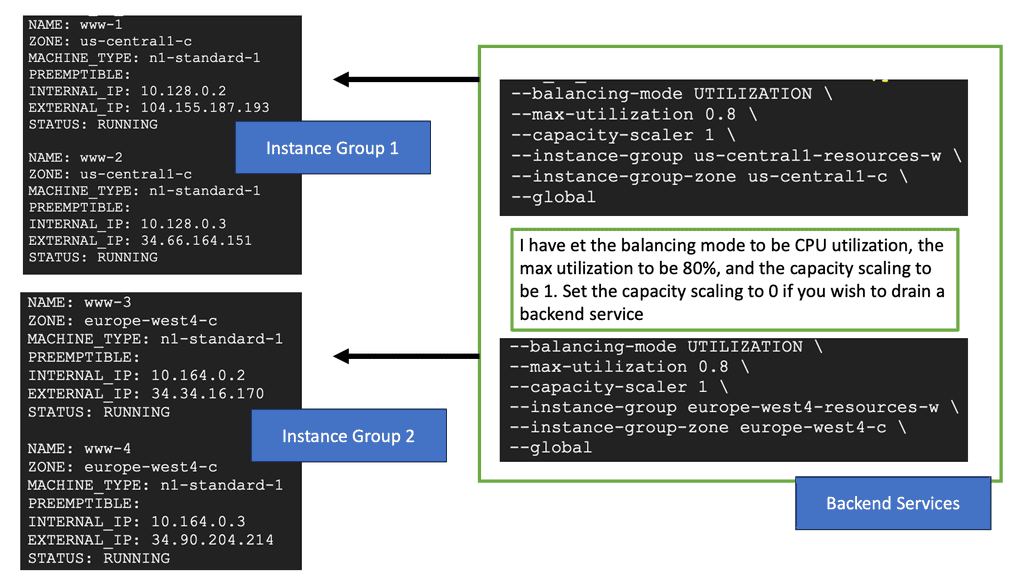
5. Scalability: Load balancers allow for easy resource scaling by adding or removing servers dynamically, ensuring optimal performance as demand fluctuates.
Types of Load Balancers
Load balancers come in different types, each catering to specific network architectures and requirements. The most common types include:
1. Hardware Load Balancers: These devices are designed for load balancing. They offer high performance and scalability and often have advanced features.
2. Software Load Balancers: These are software-based load balancers that run on standard server hardware or virtual machines. They provide flexibility and cost-effectiveness while still delivering robust load-balancing capabilities.
3. Cloud Load Balancers: Cloud service providers offer load-balancing solutions as part of their infrastructure services. These load balancers are highly scalable, automatically adapting to changing traffic patterns, and can be easily integrated into cloud environments.
GTM and LTM Load Balancing Options
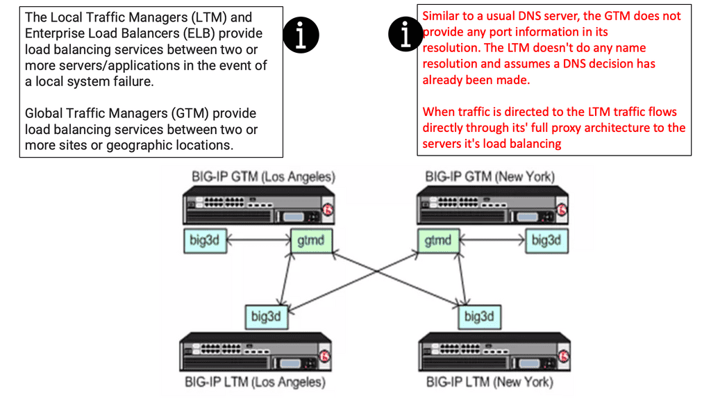
The Local Traffic Managers (LTM) and Enterprise Load Balancers (ELB) provide load-balancing services between two or more servers/applications in case of a local system failure. Global Traffic Managers (GTM) provide load-balancing services between two or more sites or geographic locations.
Local Traffic Managers, or Load Balancers, are devices or software applications that distribute incoming network traffic across multiple servers, applications, or network resources. They act as intermediaries between users and the servers or resources they are trying to access. By intelligently distributing traffic, LTMs help prevent server overload, minimize downtime, and improve system performance.
GTM and LTM Components
Before diving into the communication between GTM and LTM, let’s understand what each component does.
GTM, or Global Traffic Manager, is a robust DNS-based load-balancing solution that distributes incoming network traffic across multiple servers in different geographical regions. Its primary objective is to ensure high availability, scalability, and optimal performance by directing users to the most suitable server based on various factors such as geographic location, server health, and network conditions.
On the other hand, LTM, or Local Traffic Manager, is responsible for managing network traffic at the application layer. It works within a local data center or a specific geographic region, balancing the load across servers, optimizing performance, and ensuring secure connections.
As mentioned earlier, the most significant difference between the GTM and LTM is traffic doesn’t flow through the GTM to your servers.
GTM (Global Traffic Manager )
The GTM load balancer balances traffic between application servers across Data Centers. Using F5’s iQuery protocol for communication with other BIGIP F5 devices, GTM acts as an “Intelligent DNS” server, handling DNS resolutions based on intelligent monitors. The service determines where to resolve traffic requests among multiple data center infrastructures.
LTM (Local Traffic Manager)
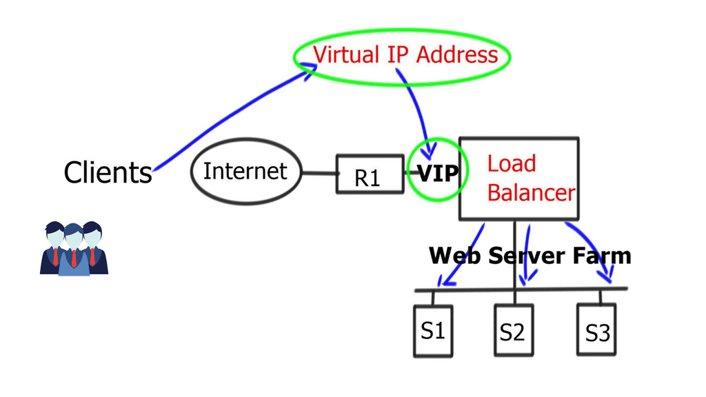
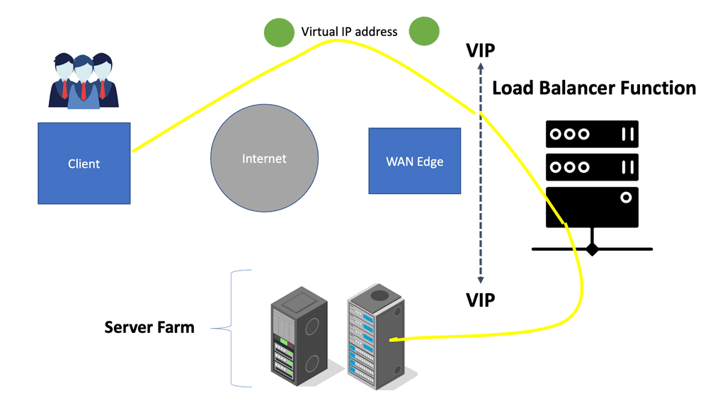
LTM balances servers and caches, compresses, persists, etc. The LTM network acts as a full reverse proxy, handling client connections. The F5 LTM uses Virtual Services (VSs) and Virtual IPs (VIPs) to configure a load-balancing setup for a service.
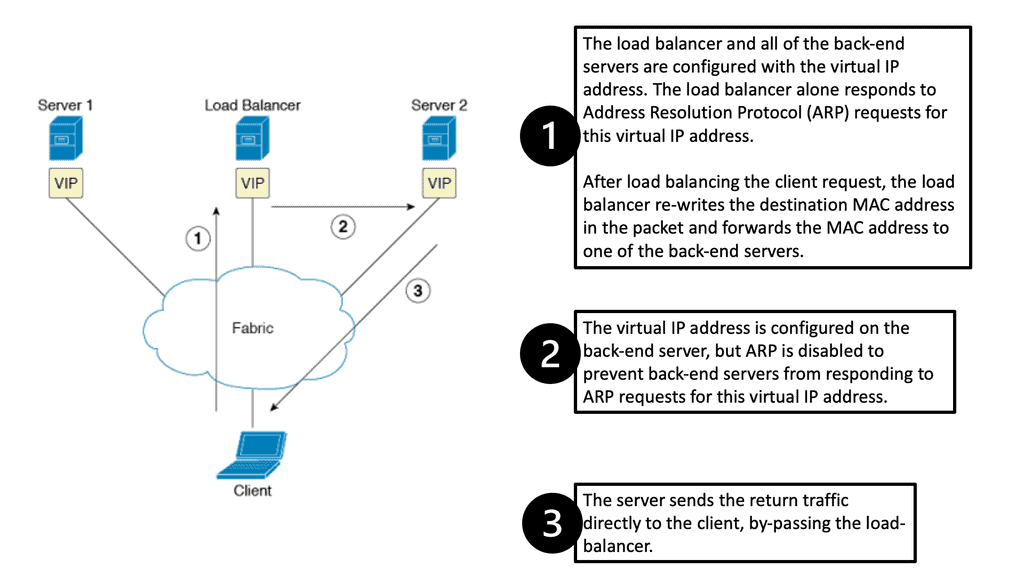
LTMs offer two load balancing methods: nPath configuration and Secure Network Address Translation (SNAT). In addition to load balancing, LTM performs caching, compression, persistence, and other functions.
Communication between GTM and LTM:
BIG-IP Global Traffic Manager (GTM) uses the iQuery protocol to communicate with the local big3d agent and other BIG-IP big3d agents. GTM monitors BIG-IP systems’ availability, the network paths between them, and the local DNS servers attempting to connect to them.
The communication between GTM and LTM occurs in three key stages:
1. Configuration Synchronization:
GTM and LTM communicate to synchronize their configuration settings. This includes exchanging information about the availability of different LTM instances, their capacities, and other relevant parameters. By keeping the configuration settings current, GTM can efficiently make informed decisions on distributing traffic.
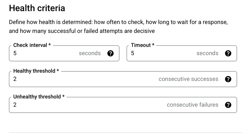
2. Health Checks and Monitoring:
GTM continuously monitors the health and availability of the LTM instances by regularly sending health check requests. These health checks ensure that only healthy LTM instances are included in the load-balancing decisions. If an LTM instance becomes unresponsive or experiences issues, GTM automatically removes it from the distribution pool, optimizing the traffic flow.
3. Dynamic Traffic Distribution:
GTM distributes incoming traffic to the most suitable LTM instances based on the configuration settings and real-time health monitoring. This ensures load balancing across multiple servers, prevents overloading, and improves the overall user experience. Additionally, GTM can reroute traffic to alternative LTM instances in case of failures or high traffic volumes, enhancing resilience and minimizing downtime.
- A key point: TCP Port 4353
LTMs and GTMs can work together or separately. Most organizations that own both modules use them together, and that’s where the real power lies.
They use a proprietary protocol called iQuery to accomplish this.
Through TCP port 4353, iQuery reports VIP availability/performance to GTMs. A GTM can then dynamically resolve VIPs that reside on an LTM. With LTMs as servers in GTM configuration, there is no need to monitor VIPs directly with application monitors since the LTM is doing that, and iQuery reports it back to the GTM.
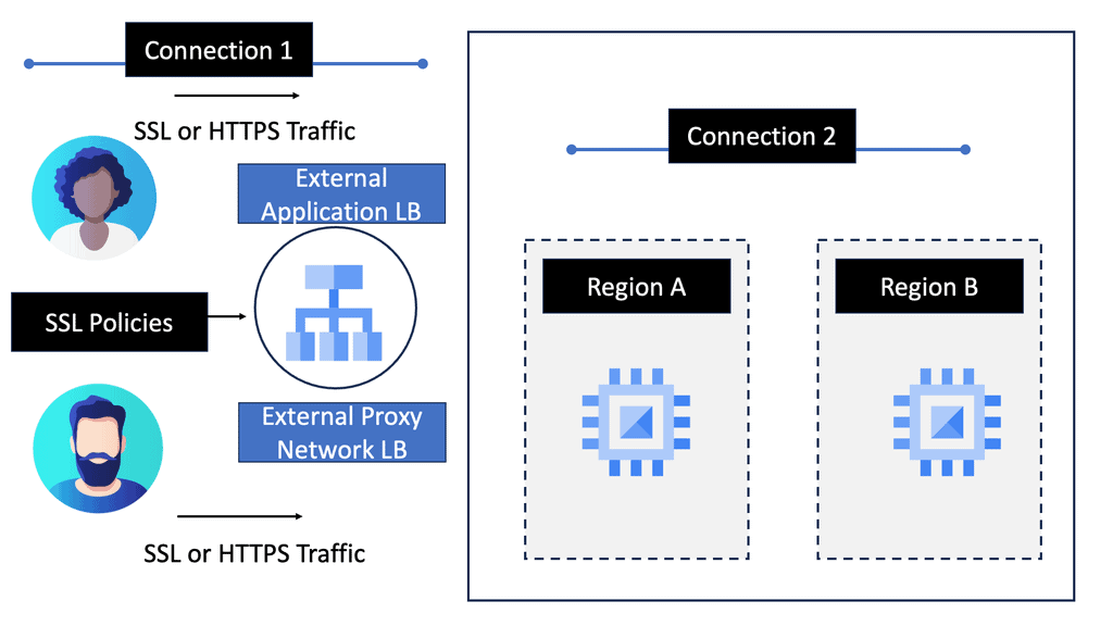
The Role of DNS With Load Balancing
The GTM load balancer offers intelligent Domain Name System (DNS) resolution capability to resolve queries from different sources to different data center locations. It loads and balances DNS queries to existing recursive DNS servers and caches the response or processes the resolution. This does two main things.
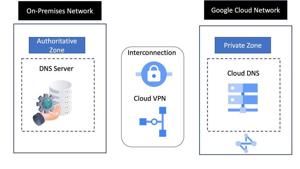
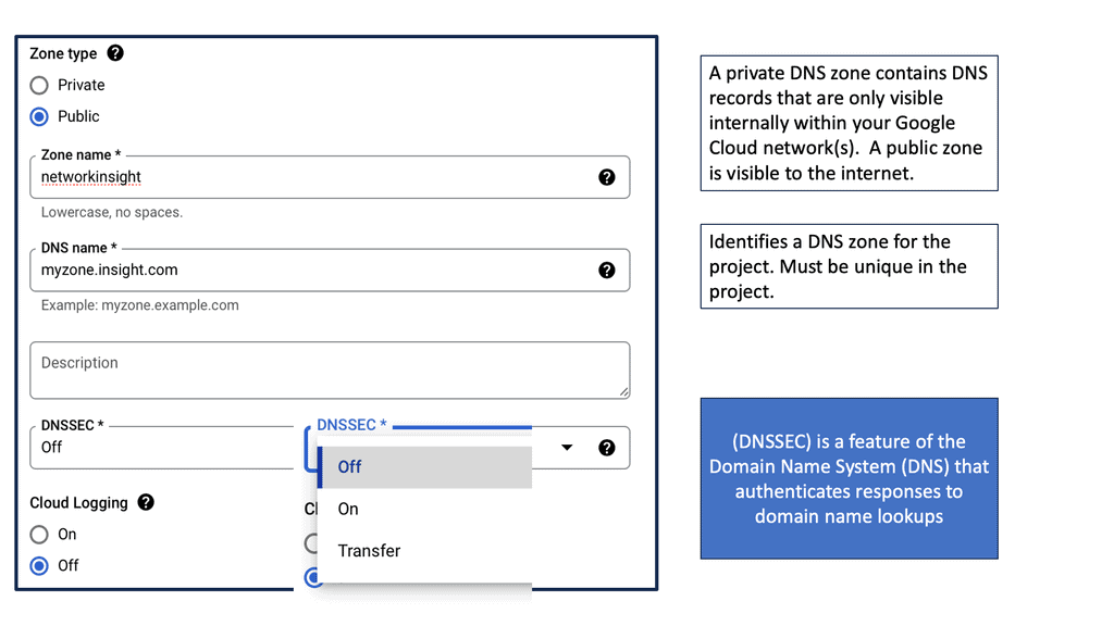
First, for security, it can enable DNS security designs and act as the authoritative DNS server or secondary authoritative DNS server web. It implements several security services with DNSSEC, allowing it to protect against DNS-based DDoS attacks.
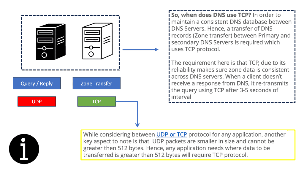
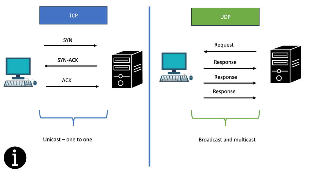
DNS relies on UDP for transport, so you are also subject to UDP control plane attacks and performance issues. DNS load balancing failover can improve performance for load balancing traffic to your data centers. DNS is much more graceful than Anycast and is a lightweight protocol.
DNS load balancing provides several significant advantages.
Adding a duplicate system may be a simple way to increase your load when you need to process more traffic. If you route multiple low-bandwidth Internet addresses to one server, the server will have a more significant amount of total bandwidth.
DNS load balancing is easy to configure. Adding the additional addresses to your DNS database is as easy as 1-2-3! It doesn’t get any easier than this!
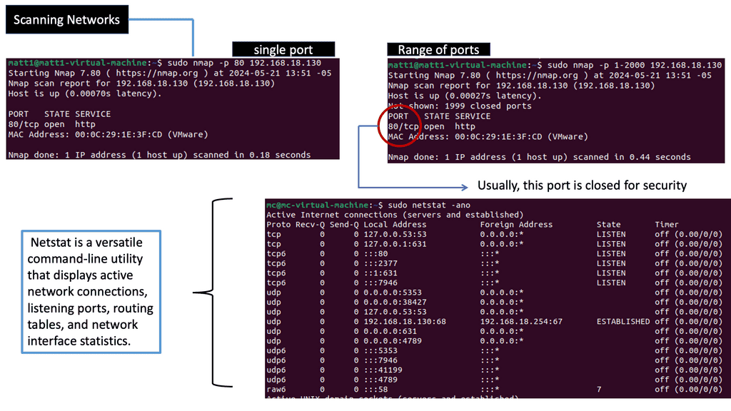
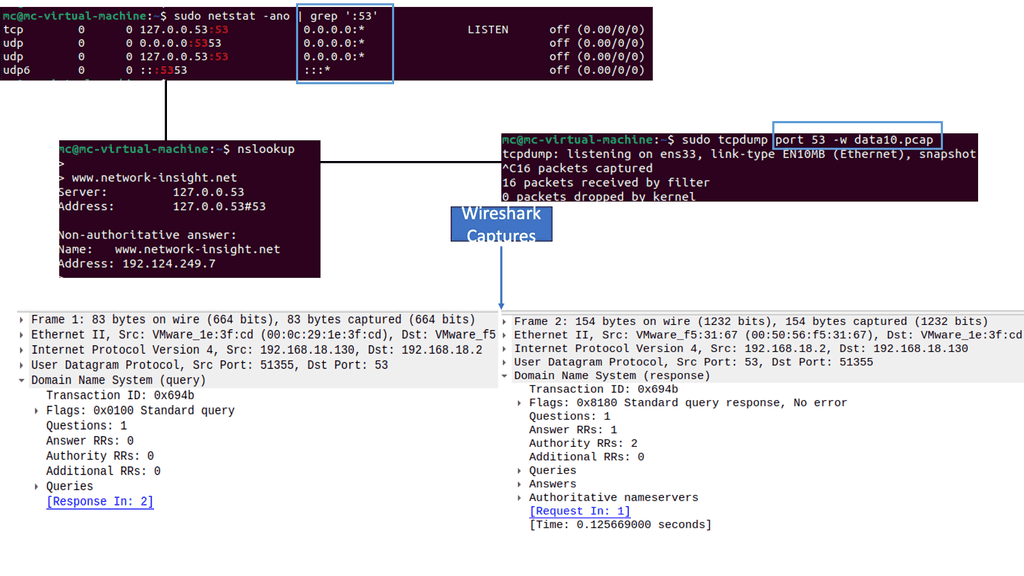
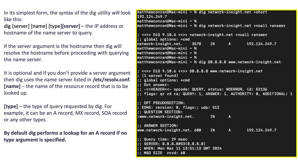
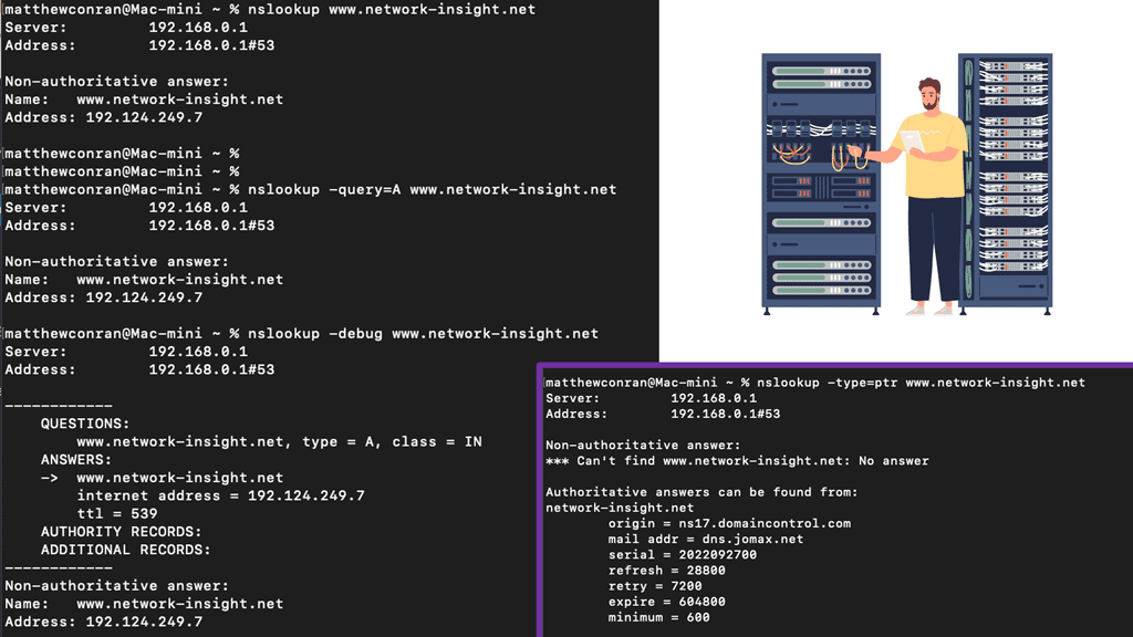
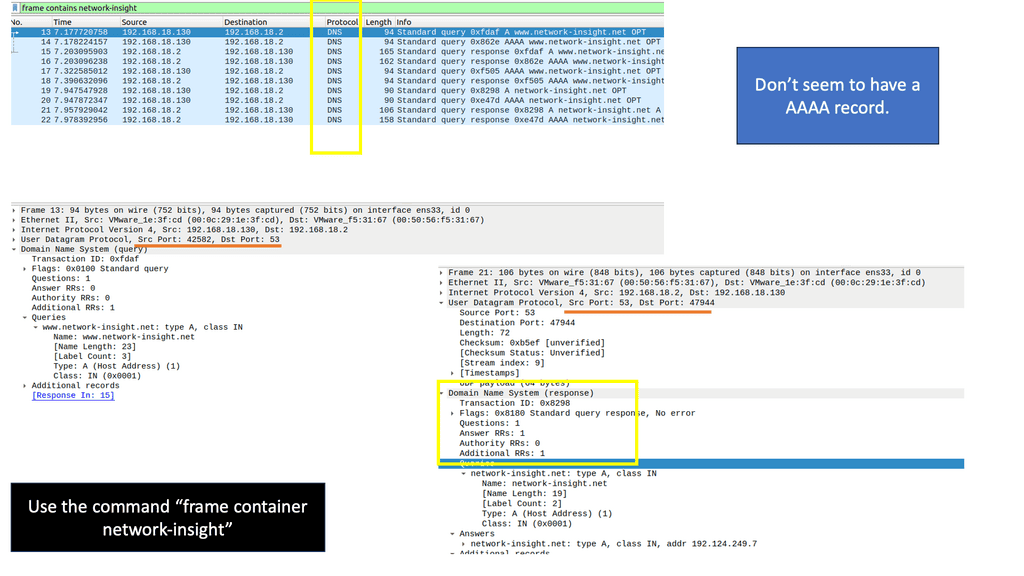
Simple to debug: You can work with DNS using tools such as dig, ping, and nslookup. In addition, BIND includes tools for validating your configuration, and all testing can be conducted via the local loopback adapter.
You will need a DNS server to have a domain name since you have a web-based system. At some point, you will undoubtedly need a DNS server. Your existing platform can be quickly extended with DNS-based load balancing!
**Issues with DNS Load Balancing**
In addition to its limitations, DNS load balancing also has some advantages.
Dynamic applications suffer from sticky behavior, but static sites rarely experience it. HTTP (and, therefore, the Web) is a stateless protocol. Chronic amnesia prevents it from remembering one request from another. To overcome this, a unique identifier accompanies each request. Identifiers are stored in cookies, but there are other sneaky ways to do this.
Through this unique identifier, your web browser can collect information about your current interaction with the website. Since this data isn’t shared between servers, if a new DNS request is made to determine the IP, there is no guarantee you will return to the server with all of the previously established information.
As mentioned previously, one in two requests may be high-intensity, and one in two may be easy. In the worst-case scenario, all high-intensity requests would go to only one server while all low-intensity requests would go to the other. This is not a very balanced situation, and you should avoid it at all costs lest you ruin the website for half of the visitors.
A fault-tolerant system. DNS load balancers cannot detect when one web server goes down, so they still send traffic to the space left by the downed server. As a result, half of all request
DNS Load Balancing Failover
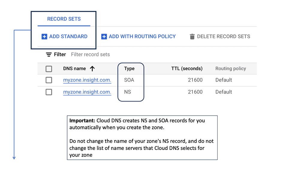
DNS load balancing is the simplest form of load balancing. As for the actual load balancing, it is somewhat straightforward in how it works. It uses a direct method called round robin to distribute connections over the group of servers it knows for a specific domain. It does this sequentially. This means going first, second, third, etc.). To add DNS load balancing failover to your server, you must add multiple A records for a domain.
GTM load balancer and LTM
DNS load balancing failover
The GTM load balancer and the Local Traffic Manager (LTM) provide load-balancing services towards physically dispersed endpoints. Endpoints are in separate locations but logically grouped in the eyes of the GTM. For data center failover events, DNS is much more graceful than Anycast. With GTM DNS failover, end nodes are restarted (cold move) into secondary data centers with a different IP address.
As long as the DNS FQDN remains the same, new client connections are directed to the restarted hosts in the new data center. The failover is performed with a DNS change, making it a viable option for disaster recovery, disaster avoidance, and data center migration.
On the other hand, stretch clusters and active-active data centers pose a separate set of challenges. In this case, other mechanisms, such as FHRP localization and LISP, are combined with the GTM to influence ingress and egress traffic flows.
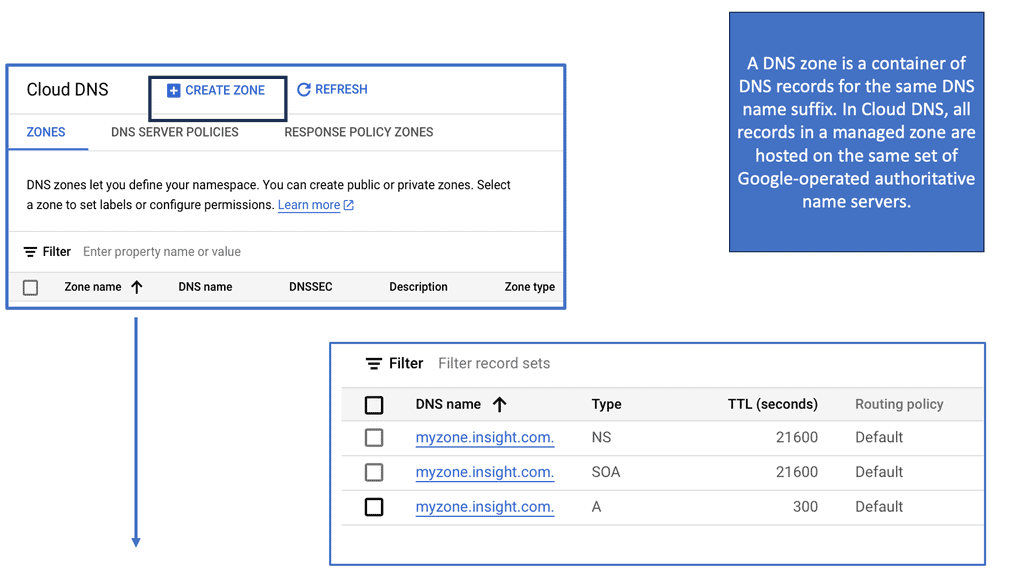
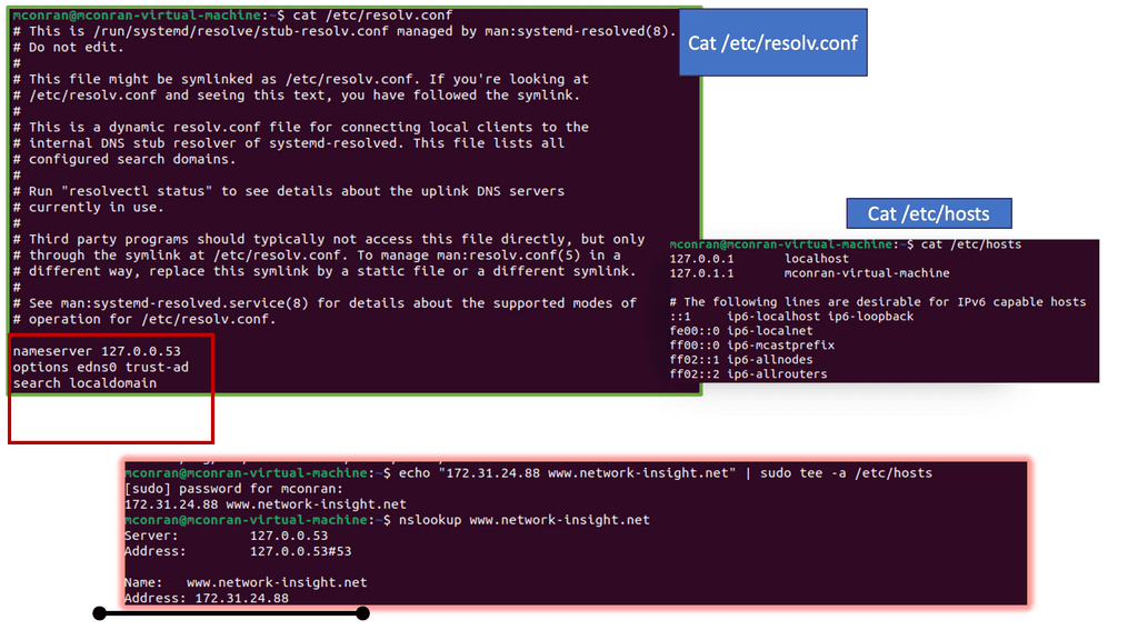
DNS Namespace Basics
Packets traverse the Internet using numeric IP addresses, not names, to identify communication devices. DNS was developed to map the IP address to a user-friendly name to make numeric IP addresses memorable and user-friendly. Employing memorable names instead of numerical IP addresses dates back to the early 1980s in ARPANET. Localhost files called HOSTS.txt mapped IP to names on all the ARPANET computers. The resolution was local, and any changes were implemented on all computers.

Example: DNS Structure
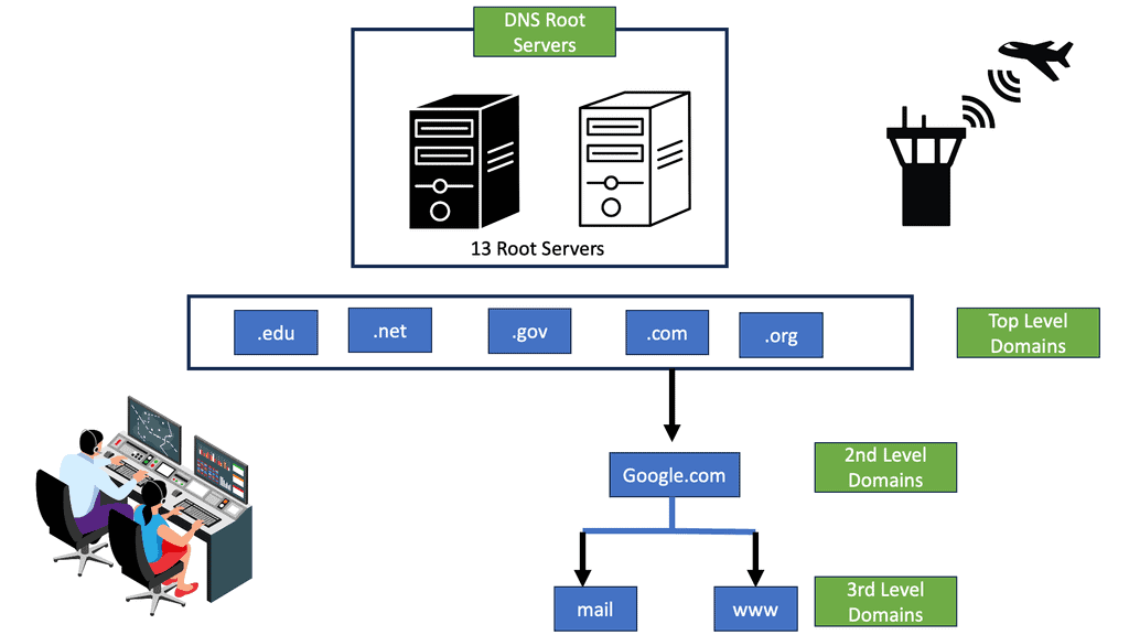
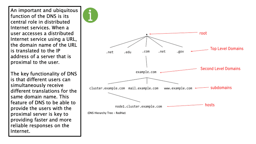
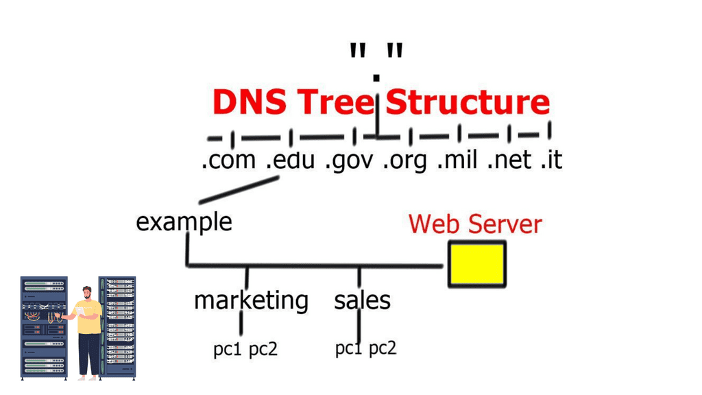
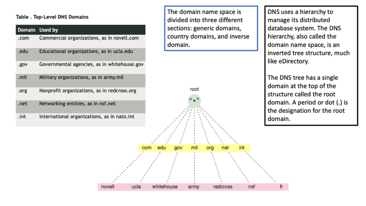
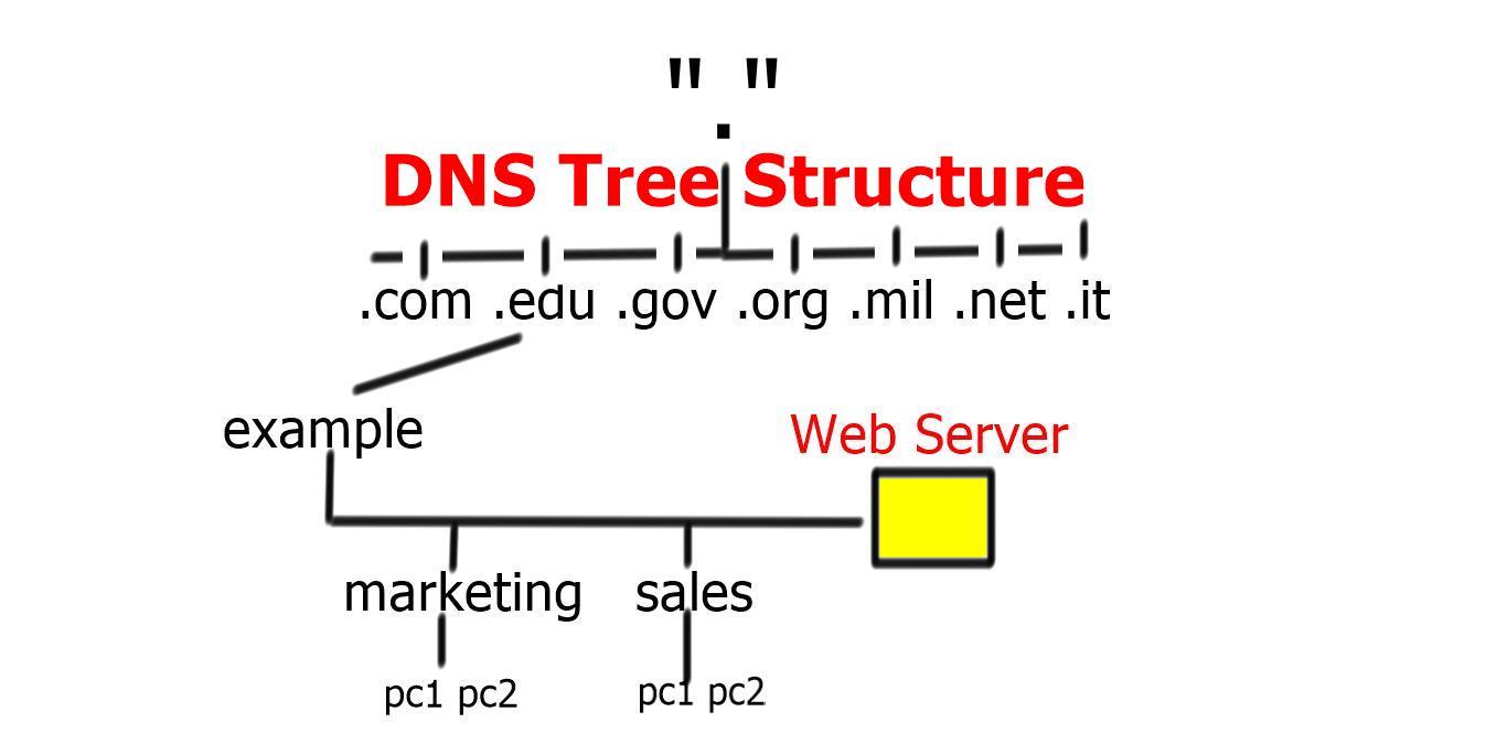
This was sufficient for small networks, but with the rapid growth of networking, a hierarchical distributed model known as a DNS namespace was introduced. The database is distributed worldwide on what’s known as DNS nameservers that consist of a DNS structure. It resembles an inverted tree, with branches representing domains, zones, and subzones.
At the very top of the domain is the “root” domain, and then further down, we have Top-Level domains (TLD), such as .com or .net. and Second-Level domains (SLD), such as www.network-insight.net.
The IANA delegates management of the TLD to other organizations such as Verisign for.COM and. NET. Authoritative DNS nameservers exist for each zone. They hold information about the domain tree structure. Essentially, the name server stores the DNS records for that domain.
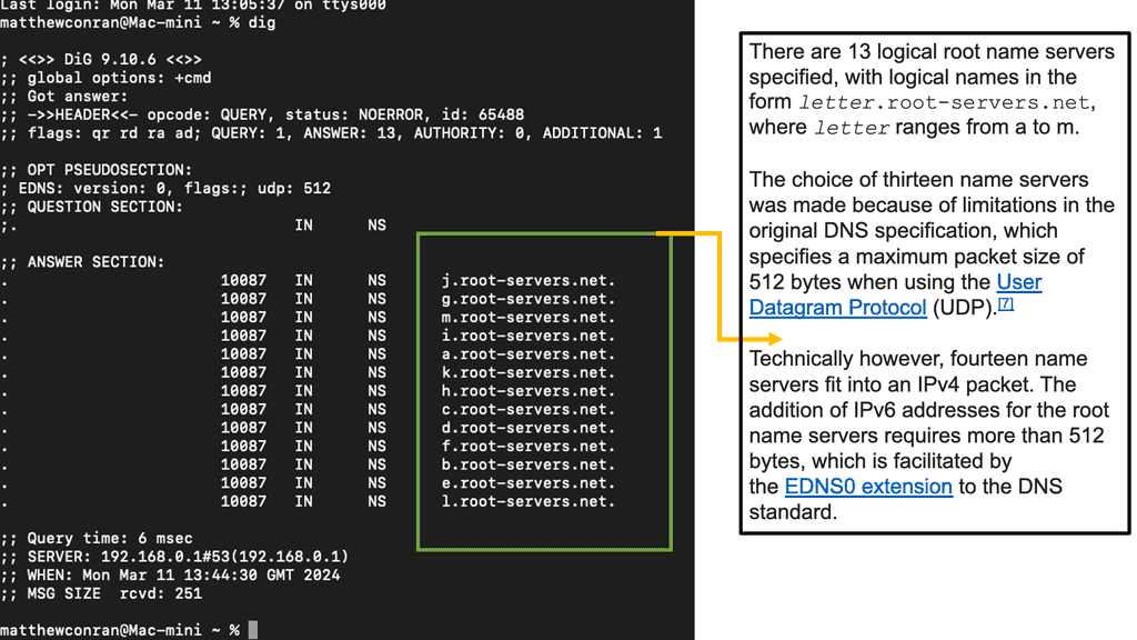
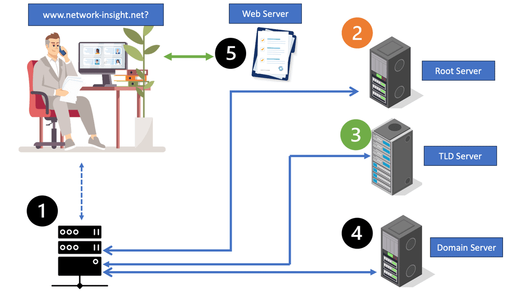
You interact with the DNS infrastructure with the process known as RESOLUTION. First, end stations request a DNS to their local DNS (LDNS). If the LDNS supports caching and has a cached response for the query, it will respond to the client’s requests.
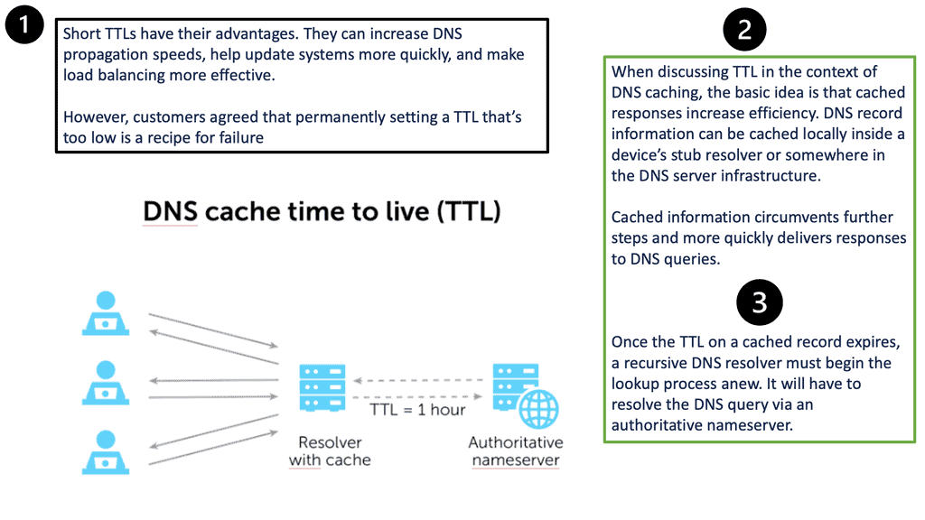
DNS caching stores DNS queries for some time, which is specified in the DNS TTL. Caching improves DNS efficiency by reducing DNS traffic on the Internet. If the LDNS doesn’t have a cached response, it will trigger what is known as the recursive resolution process.
Next, the LDNS queries the authoritative DNS server in the “root” zones. These name servers will not have the mapping in their database but will refer the request to the appropriate TLD. The process continues, and the LDNS queries the authoritative DNS in the appropriate.COM .NET or. ORG zones. The method has many steps and is called “walking a tree.” However, it is based on a quick transport protocol (UDP) and takes only a few milliseconds.
DNS Load Balancing Failover Key Components
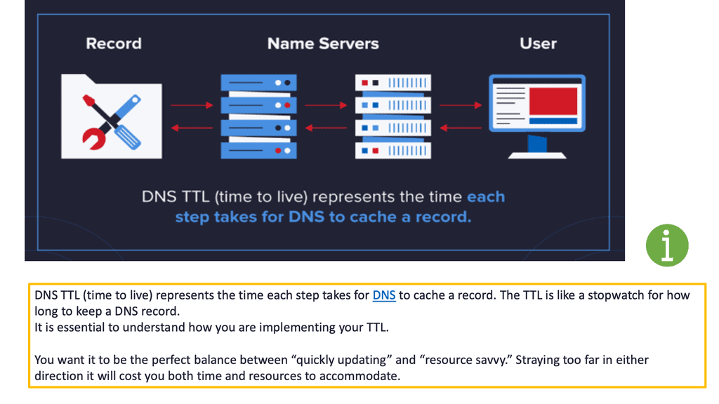
DNS TTL
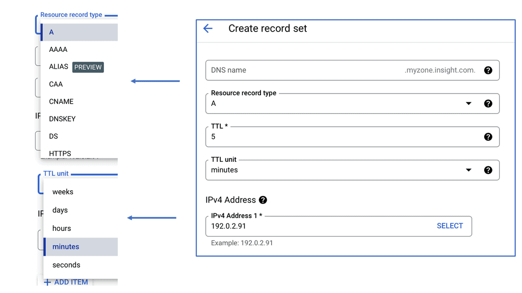
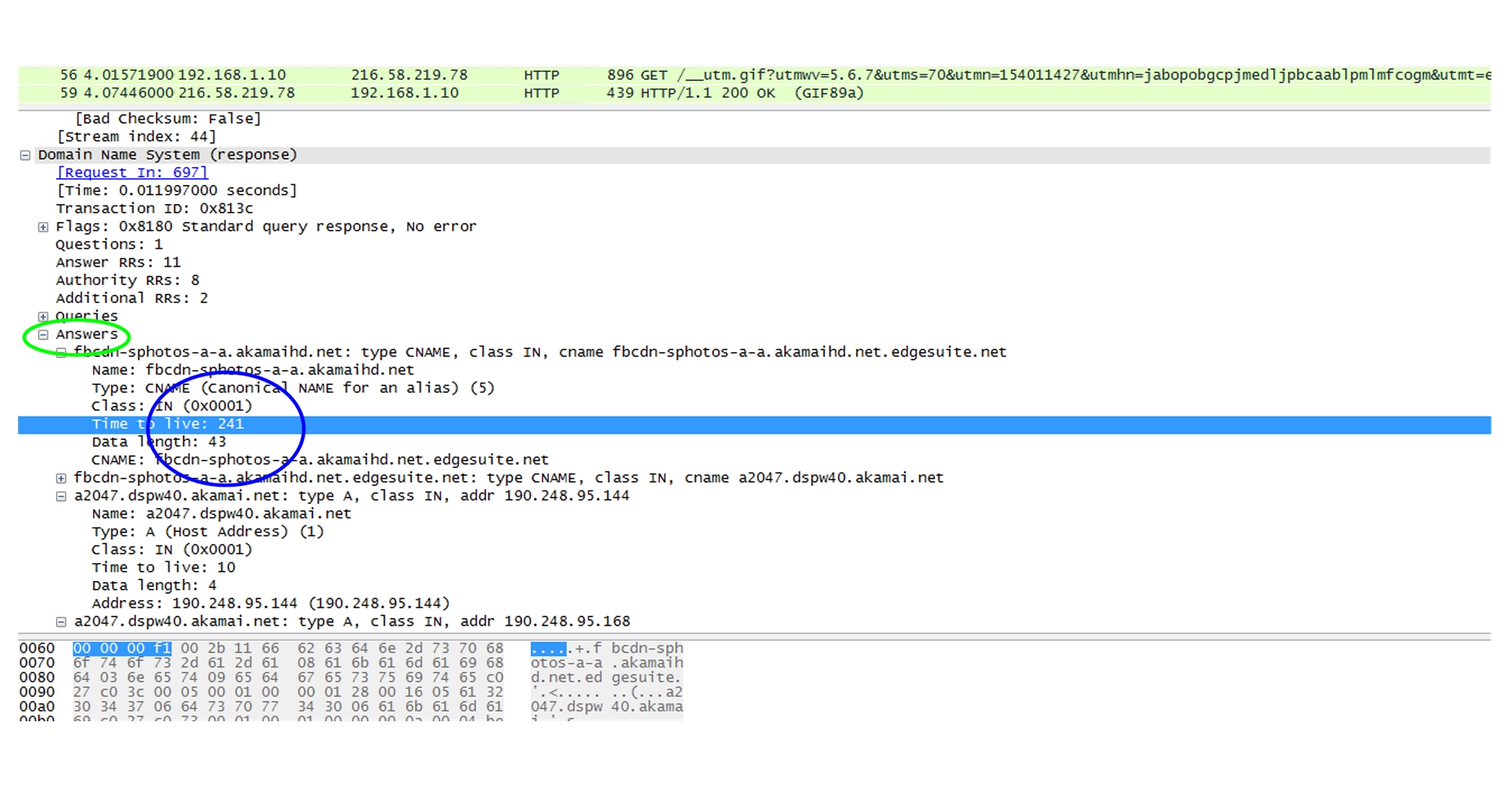
Once the LDNS gets a positive result, it caches the response for some time, referenced by the DNS TTL. The DNS TTL setting is specified in the DNS response by the authoritative nameserver for that domain. Previously, an older and common TTL value for DNS was 86400 seconds (24 hours).
This meant that if there were a change of record on the DNS authoritative server, the DNS servers around the globe would not register that change for the TTL value of 86400 seconds.
This was later changed to 5 minutes for more accurate DNS results. Unfortunately, TTL in some end hosts’ browsers is 30 minutes, so if there is a failover data center event and traffic needs to move from DC1 to DC2, some ingress traffic will take time to switch to the other DC, causing long tails.
DNS pinning and DNS cache poisoning
Web browsers implement a security mechanism known as DNS pinning, where they refuse to take low TTL as there are many security concerns with low TTL settings, such as cache poisoning. Every time you read from the DNS namespace, there is potential DNS cache poisoning and a DNS reflection attack.
Because of this, all browser companies ignored low TTL and implemented their aging mechanism, which is about 10 minutes.
In addition, there are embedded applications that carry out a DNS lookup only once when you start the application, for example, a Facebook client on your phone. During data center failover events, this may cause a very long tail, and some sessions may time out.
GTM Load Balancer and GTM Listeners
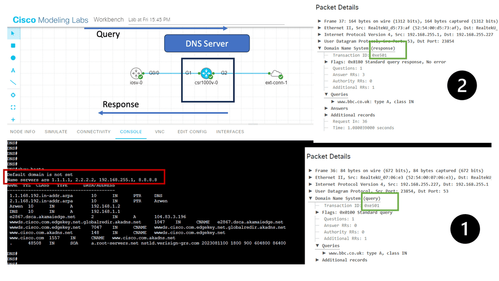
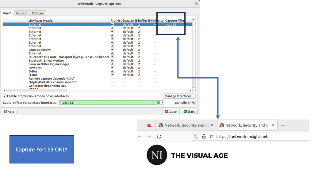
The first step is to configure GTM Listeners. A listener is a DNS object that processes DNS queries. It is configured with an IP address and listens to traffic destined to that address on port 53, the standard DNS port. It can respond to DNS queries with accelerated DNS resolution or GTM intelligent DNS resolution.
GTM intelligent Resolution is also known as Global Server Load Balancing (GSLB) and is just one of the ways you can get GTM to resolve DNS queries. It monitors a lot of conditions to determine the best response.
The GTM monitors LTM and other GTMs with a proprietary protocol called IQUERY. IQUERY is configured with the bigip_add utility. It’s a script that exchanges SSL certificates with remote BIG-IP systems. Both systems must be configured to allow port 22 on their respective self-IPs.
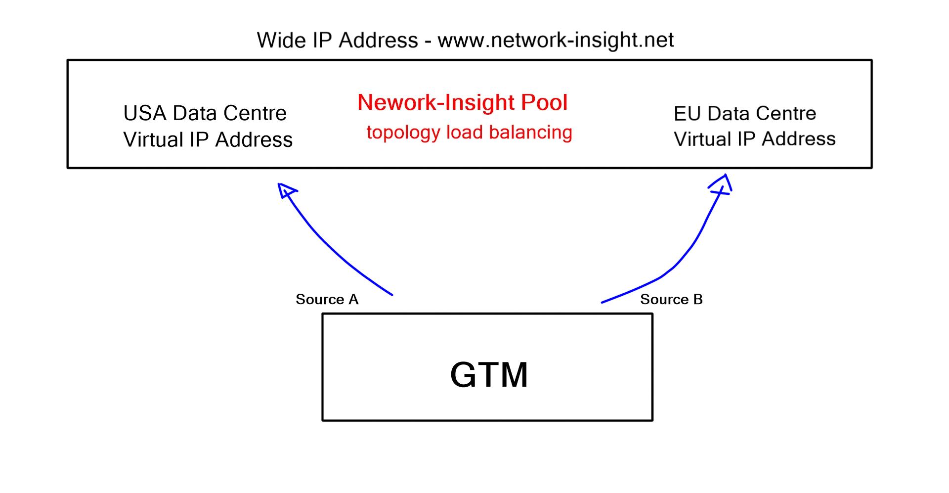
The GTM allows you to group virtual servers, one from each data center, into a pool. These pools are then grouped into a larger object known as a Wide IP, which maps the FQDN to a set of virtual servers. The Wide IP may contain Wild cards.
Load Balancing Methods
When the GTM receives a DNS query that matches the Wide IP, it selects the virtual server and sends back the response. Several load balancing methods (Static and Dynamic) are used to select the pool; the default is round-robin. Static load balancing includes round-robin, ratio, global availability, static persists, drop packets, topology, fallback IP, and return to DNS.
Dynamic load balancing includes round trip time, completion time, hops, least connections, packet rate, QoS, and kilobytes per second. Both methods involve predefined configurations, but dynamic considers real-time events.
For example, topology load balancing allows you to select a DNS query response based on geolocation information. Queries are resolved based on the resource’s physical proximity, such as LDNS country, continent, or user-defined fields. It uses an IP geolocation database to help make the decisions. It helps service users with correct weather and news based on location. All this configuration is carried out with Topology Records (TR).
Anycast and GTM DNS for DC failover
Anycast means you advertise the same address from multiple locations. It is a viable option when data centers are geographically far apart. Anycast solves the DNS problem, but we also have a routing plane to consider. Getting people to another DC with Anycast can take time and effort.
It’s hard to get someone to go to data center A when the routing table says go to data center B. The best approach is to change the actual routing. As a failover mechanism, Anycast is not as graceful as DNS migration with F5 GTM.
Generally, if session disruption is a viable option, go for Anycast. Web applications would be OK with some session disruption. HTTP is stateless, and it will just resend. However, other types of applications might not be so tolerant. If session disruption is not an option and graceful shutdown is needed, you must use DNS-based load balancing. Remember that you will always have long tails due to DNS pinning in browsers, and eventually, some sessions will be disrupted.
Scale-Out Applications
The best approach is to do a fantastic scale-out application architecture. Begin with parallel application stacks in both data centers and implement global load balancing based on DNS. Start migrating users to the other data center, and when you move all the other users, you can shut down the instance in the first data center. It is much cleaner and safer to do COLD migrations. Live migrations and HOT moves (keep sessions intact) are challenging over Layer 2 links.
You need a different IP address. You don’t want to have stretched VLANs across data centers. It’s much easier to make a COLD move, change the IP, and then use DNS. The load balancer config can be synchronized to vCenter, so the load balancer definitions are updated based on vCenter VM groups.
Another reason for failures in data centers during scale-outs could be the lack of airtight sealing, otherwise known as hermetic sealing. Not having an efficient seal brings semiconductors in contact with water vapor and other harmful gases in the atmosphere. As a result, ignitors, sensors, circuits, transistors, microchips, and much more don’t get the protection they require to function correctly.
Data and Database Challenges
The main challenge with active-active data centers and failover events is with your actual DATA and Databases. If data center A fails, how accurate will your data be? You cannot afford to lose any data if you are running a transaction database.
Resilience is achieved by storage or database-level replication that employs log shipping or distribution between two data centers with a two-phase commit. Log shipping has an RPO of non-zero, as transactions could happen a minute before. A two-phase commit synchronizes multiple copies of the database but can slow down due to latency.
GTM Load Balancer is a robust solution for optimizing website performance and ensuring high availability. With its advanced features and intelligent traffic routing capabilities, businesses can enhance their online presence, improve user experience, and handle growing traffic demands. By leveraging the power of GTM Load Balancer, online companies can stay competitive in today’s fast-paced digital landscape.
Efficient communication between GTM and LTM is essential for businesses to optimize network traffic management. By collaborating seamlessly, GTM and LTM provide enhanced performance, scalability, and high availability, ensuring a seamless experience for end-users. Leveraging this powerful duo, businesses can deliver their services reliably and efficiently, meeting the demands of today’s digital landscape.
Closing Points on F5 GTM
Global Traffic Management (GTM) load balancing is a crucial component in ensuring your web applications remain accessible, efficient, and resilient on a global scale. With the rise of digital businesses, having a robust and dynamic load balancing strategy is more important than ever. In this blog, we will explore the intricacies of GTM load balancing, focusing on the capabilities provided by F5, a leader in application delivery networking.
F5’s Global Traffic Manager (GTM) is a powerful tool that optimizes the distribution of user requests by directing them to the most appropriate server based on factors such as location, server performance, and user requirements. The goal is to reduce latency, improve response times, and ensure high availability. F5 achieves this through intelligent DNS resolution and real-time network health monitoring.
1. **Intelligent DNS Resolution**: F5 GTM uses advanced algorithms to resolve DNS queries by considering factors such as server load, geographical location, and network latency. This ensures that users are directed to the server that can provide the fastest and most reliable service.
2. **Comprehensive Health Monitoring**: One of the standout features of F5 GTM is its ability to perform continuous health checks on servers and applications. This allows it to detect failures promptly and reroute traffic to healthy servers, minimizing downtime.
3. **Enhanced Security**: F5 GTM incorporates robust security measures, including DDoS protection and SSL/TLS encryption, to safeguard data and maintain the integrity of web applications.
4. **Scalability and Flexibility**: With F5 GTM, businesses can easily scale their operations to accommodate increased traffic and expand to new locations without compromising performance or reliability.
Integrating F5 GTM into your existing IT infrastructure requires careful planning and execution. Here are some steps to ensure a smooth implementation:
– **Assessment and Planning**: Begin by assessing your current infrastructure needs and identifying areas that require load balancing improvements. Plan your GTM strategy to align with your business goals.
– **Configuration and Testing**: Configure F5 GTM settings based on your requirements, such as setting up DNS zones, health monitors, and load balancing policies. Conduct thorough testing to ensure all components work seamlessly.
– **Deployment and Monitoring**: Deploy F5 GTM in your production environment and continuously monitor its performance. Use F5’s comprehensive analytics tools to gain insights and make data-driven decisions.