
Network Connectivity
Modern applications depend on connectivity.
Whether a user is opening a web application, a Kubernetes workload is communicating with another service, a database is replicating across a data centre, or a cloud platform is reaching an on-premises system, the underlying requirement is the same: data must move reliably from one endpoint to another.
That sounds simple. In modern infrastructure, it rarely is.
A packet may pass through switches, routers, routing domains, security boundaries, load balancers, tunnels, overlays and cloud networks before reaching its destination. Along the way, the network must resolve neighbours, select routes, apply policy, enforce security controls, handle MTU constraints and establish the appropriate transport or application session.
Connectivity is therefore much more than having an IP address and a reachable interface.
A useful way to understand modern networking is as a chain of dependent decisions:
CONNECT → RESOLVE → ROUTE → SECURE → TRANSPORT → DELIVER → OBSERVE
Each stage depends on the others. An interface must be operational before traffic can leave a host. Neighbour discovery must succeed before the next hop can be reached. Routing must select a valid path. Security policy must permit the traffic. NAT, tunnelling or segmentation may alter how the packet travels. Transport protocols must establish communication where required, and the application must ultimately be available and responding.
A failure at any one of these stages can produce the same familiar symptom:
“The application is unreachable.”
The challenge for a network engineer is determining where the failure actually occurred.
Traditional networking is often taught as a collection of individual technologies: Ethernet, VLANs, IPv4, IPv6, ARP, TCP, UDP, OSPF, BGP, firewalls and NAT. These technologies remain fundamental, but production connectivity is created by their interaction.
A packet can move from a container through a virtual interface, across an Open vSwitch datapath, through a Kubernetes service, across a VXLAN overlay, through an EVPN-controlled fabric, into a WAN, across a cloud routing domain and eventually toward an application endpoint.
The individual protocols have not disappeared. They have become layers within a much larger connectivity system.
Modern networks also require an understanding of the relationship between the control plane and the data plane. The control plane determines what should happen. Routing protocols exchange information, calculate paths, apply policy and build routing state. The data plane executes those decisions using forwarding tables, neighbour information, ACLs, firewall rules, NAT state and switching or routing pipelines.
This distinction becomes particularly important when troubleshooting.
A routing protocol can be healthy while forwarding is incorrect. A route can exist while an ACL blocks the packet. A TCP session can fail even though IP connectivity works. A service can be unreachable even though every network hop appears healthy.
Control-plane correctness does not automatically guarantee application connectivity.
Modern connectivity failures are rarely caused by one technology in isolation. Incorrect addressing, VLAN configuration, missing ARP or IPv6 neighbour discovery, routing decisions, asymmetric paths, VRF segmentation, BGP or IGP policy, ACLs, firewalls, NAT, MTU problems, DNS, Kubernetes networking, cloud route tables, overlay tunnels and application health can all influence the final result.
This creates an important engineering principle:
Troubleshoot connectivity as a chain of dependencies, not as a collection of isolated devices.
Instead of asking only, “Is the router working?”, the better questions are:
Where is the packet now?
What is the next hop?
Which control plane made the decision?
What does the data plane actually do?
Which policy could stop the packet?
Where does the packet disappear?
What evidence proves the failure?
That mindset scales from a small LAN to a data-centre fabric, a WAN, a cloud environment or a Kubernetes platform.
This article takes a practical approach to understanding that connectivity chain. Rather than treating networking as a collection of static diagrams, the interactive sections allow you to follow what happens to traffic as it moves through a modern network.
You will examine how packets are encapsulated and forwarded, how routing and neighbour resolution influence the next hop, how security and transport affect connectivity, how routing control planes build forwarding state, and how cloud-native platforms introduce additional networking layers.
The later investigations deliberately introduce failures so that connectivity can be analysed from the perspective of an engineer troubleshooting a real system.
The objective is not simply to memorise protocols.
It is to develop a repeatable way of thinking:
What is the source? What is the destination? What is the next hop? Which decision was made? Where did the packet stop? Why did it stop? What evidence proves it?
Modern infrastructure is no longer a collection of isolated networks. It is a distributed connectivity fabric spanning hosts, switches, routers, security systems, WANs, data centres, cloud platforms, containers and applications.
Understanding how those layers interact is one of the most important foundations for modern network engineering.
The goal is simple:
Follow the packet. Understand the decision. Find the failure. Prove the result.
Highlights: Network Connectivity
Connectivity Engineering Journey
Move from packet fundamentals through routing, cloud-native networking and finally into structured connectivity investigation.
Understand how a packet is created, encapsulated, switched, routed and delivered across a network.
Follow the dependencies between addressing, neighbour discovery, ACLs, firewalls, NAT, MTU and transport.
See how routing protocols become forwarding state and how VRFs, overlays and fabrics extend connectivity.
Trace traffic through namespaces, veth pairs, CNI networking, datapaths, services and policy.
Investigate an unreachable application by proving where the connectivity chain breaks and why.
How Connectivity Is Built
Before following an individual packet, understand the chain of decisions that allows an application to communicate. Select a layer to see what it contributes to the end-to-end connectivity path.
Application
Packet & Protocol Explorer
Follow one packet from application data through Ethernet, switching, routing and final delivery.
Network Connectivity
Modern network connectivity is not simply the ability to reach an IP address.
A successful network flow depends on a chain of decisions and transformations that begin at the endpoint and continue through switching, routing, security, transport and application services.
A useful engineering model is:
CONNECT → RESOLVE → ROUTE → SECURE → TRANSPORT → DELIVER → OBSERVE
Each stage can fail independently.
A host can have a valid IP address but no Layer 2 connectivity. A gateway can be reachable while the destination route is missing. A route can exist while a firewall blocks the flow. TCP can establish successfully while the application itself fails.
Understanding connectivity therefore requires understanding the complete forwarding path rather than testing a single protocol in isolation.
The Modern Connectivity Fabric
A modern enterprise flow may cross several network domains before an application response reaches the user:
Endpoint → Access Network → Switching → Routing → Security → WAN/Cloud → Platform → Application
The physical path may involve Ethernet or Wi-Fi at the edge, VLANs and trunks inside the local network, routed interfaces and VRFs through the infrastructure, firewalls and security policies at trust boundaries, and overlays such as VXLAN across a data-centre fabric.
The destination may then reside inside a cloud VPC, a Kubernetes cluster, a virtual machine, a container or a distributed application.
Connectivity is therefore better understood as a fabric of forwarding domains and control planes than as a single network.
End-to-End Connectivity Model
| Layer / Domain | Primary Function | Typical Technologies |
|---|---|---|
| Endpoint | Generates and receives traffic | OS networking, sockets, NIC |
| Access | Provides local attachment | Ethernet, Wi-Fi, VLAN |
| Switching | Moves frames within Layer 2 | MAC tables, 802.1Q, STP |
| Routing | Selects Layer 3 paths | OSPF, IS-IS, BGP, static routes |
| Segmentation | Separates routing domains | VRF, VLAN, tenant networks |
| Security | Applies traffic policy | ACL, firewall, security groups |
| Transport | Establishes communication | TCP, UDP, QUIC |
| WAN / Cloud | Extends connectivity domains | VPN, SD-WAN, VPC, transit |
| Platform | Connects workloads | Kubernetes, CNI, service networking |
| Application | Provides the actual service | HTTP, TLS, DNS, APIs |
The important point is that these layers are related but not interchangeable.
Routing does not replace firewall policy. A successful ping does not prove that an HTTPS application works. DNS resolution does not prove that the destination port is reachable.
Each layer provides evidence about a different part of the connectivity chain.
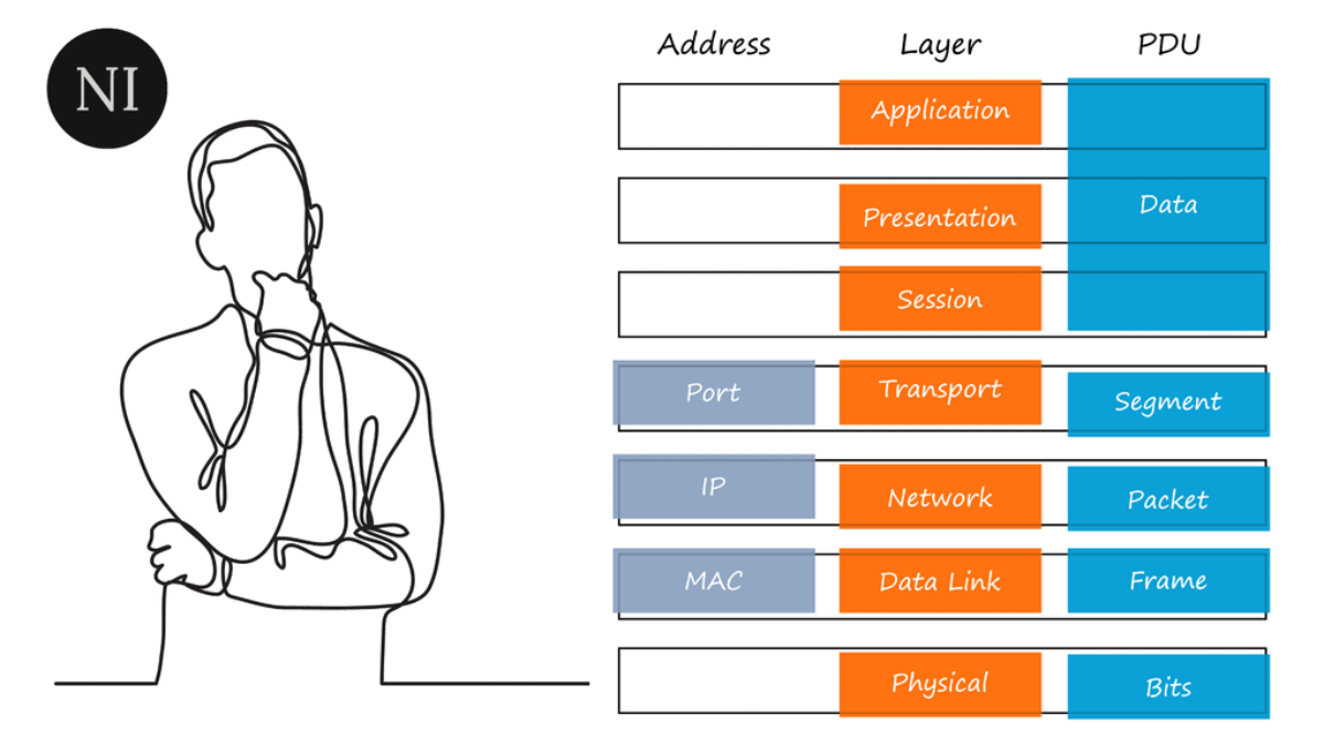
What Actually Happens to a Packet
When an application sends data, the application does not normally construct an Ethernet frame itself.
Instead, data is progressively encapsulated as it moves down the networking stack.
Application data
↓
TCP segment / UDP datagram
↓
IP packet
↓
Ethernet frame
↓
Physical or virtual transmission
At the destination, the process is reversed through decapsulation.
Frame → IP packet → Transport data → Application data
This distinction is important when troubleshooting because each layer exposes different failure conditions.
For example:
An Ethernet problem may prevent the frame from reaching the next hop.
An IP routing problem may send the packet toward the wrong destination.
A firewall may intentionally discard the packet.
TCP may fail even though IP connectivity exists.
TLS may fail after TCP succeeds.
The application may return an error even though every lower layer is functioning correctly.
Packet Anatomy
An IPv4 packet carried inside an Ethernet frame can contain information such as:
Ethernet
Source MAC address
Destination MAC address
802.1Q VLAN tag, when present
EtherType
IPv4
Source IP address
Destination IP address
TTL
Protocol
Fragmentation fields
Header checksum
TCP
Source port
Destination port
Sequence number
Acknowledgement number
Window
TCP flags
MSS and other negotiated options
The fields are used for different decisions.
The destination MAC address is relevant to the local Layer 2 hop.
The destination IP address identifies the Layer 3 destination.
The TCP destination port identifies the transport service.
This is why a routed packet can change its Ethernet header at every Layer 3 hop while its destination IP normally remains unchanged from end to end.
Encapsulation and Decapsulation
Consider a client accessing:
10.20.30.40:443
The application generates data for an HTTPS session.
The host creates a TCP segment with:
Source Port → Ephemeral client port
Destination Port → 443
The TCP segment is placed inside an IP packet:
Source IP → Client address
Destination IP → 10.20.30.40
The IP packet is then placed inside an Ethernet frame.
If the destination is on another subnet, the Ethernet destination is normally the MAC address of the local next-hop gateway, not the MAC address of 10.20.30.40.
The router receives the frame, removes the Layer 2 header, examines the destination IP address, performs a forwarding lookup and constructs a new Layer 2 frame for the next link.
This process repeats at each routed hop.
The key engineering principle is:
Layer 2 delivers the frame to the next local hop. Layer 3 determines where the packet needs to go.
Switching and Layer 2 Connectivity
Before routing can occur, many network flows must first cross a Layer 2 segment.
Ethernet switches build forwarding decisions using learned MAC addresses.
When a frame arrives, a switch can conceptually perform this sequence:
Receive frame
→ Learn source MAC
→ Identify VLAN
→ Search destination MAC
→ Apply forwarding policy
→ Select egress interface
→ Transmit frame
The switch therefore maintains a forwarding database containing relationships such as:
MAC address → VLAN → switch port
This table is learned dynamically from observed traffic.
MAC Learning
Suppose a frame arrives from host A:
AA:AA:AA:AA:AA:01
on switch port 10.
The switch can learn:
AA:AA:AA:AA:AA:01 → Port 10
If host B is already known on port 20, traffic destined for B can be forwarded directly to port 20.
If the destination MAC is unknown, the switch may flood the frame within the relevant Layer 2 broadcast domain, subject to the VLAN and forwarding rules.
This is one reason large Layer 2 domains can become operationally complex.
Unknown unicast traffic, broadcast traffic and multicast traffic can all consume resources across the same domain.
VLANs and Trunks
VLANs provide logical Layer 2 segmentation.
An access interface normally associates an endpoint with a particular VLAN.
A trunk can carry multiple VLANs between network devices using IEEE 802.1Q tagging.
Conceptually:
Access Port
Endpoint → VLAN 20
Trunk
VLAN 10
VLAN 20
VLAN 30
VLAN 40
The VLAN identifier allows switches to keep otherwise shared physical infrastructure logically separated.
However, a VLAN is not a complete security boundary by itself.
When traffic must move between VLANs, a Layer 3 gateway or routing function is required.
Layer 2 Failure Domains
Layer 2 connectivity introduces its own failure modes.
Examples include:
Incorrect VLAN assignment
Trunk allowed-VLAN mismatch
Native VLAN mismatch
MAC learning problems
Layer 2 loops
STP convergence
Broadcast storms
Unknown-unicast flooding
Port security violations
Physical interface errors
A host can therefore have a perfectly configured IP address while remaining unreachable because its Ethernet frame never reaches the correct Layer 3 gateway.
Routing and Forwarding
Routing answers a fundamental question:
Where should this IP packet go next?
The answer is not normally determined by the application.
It is determined by the network’s routing and forwarding mechanisms.
A router can maintain many routes to different destinations. These routes may originate from:
Connected interfaces
Static configuration
OSPF
IS-IS
EIGRP
BGP
Policy-based mechanisms
Other routing sources
The routing system must determine which route should become the active path.
The forwarding system then uses that decision for individual packets.
Control Plane and Data Plane
The distinction between control plane and data plane is fundamental.
Control Plane
The control plane learns and calculates reachability.
Examples:
OSPF neighbour relationships
IS-IS adjacencies
BGP sessions
Static routes
Route policies
BGP path selection
The result contributes to the device’s routing information.
Data Plane
The data plane forwards individual packets.
It uses the resulting forwarding information to determine:
Destination → Prefix match → Next hop → Egress interface
The control plane can therefore be thought of as determining what should be reachable, while the data plane determines how each packet is actually forwarded.
RIB → Best Route → FIB
A simplified routing process looks like this:
Routing Information Sources
↓
RIB
↓
Best Route Selection
↓
FIB
↓
Longest Prefix Match
↓
Next Hop
↓
Adjacency
↓
Forwarding
The RIB represents the routing information used by the control plane.
The best-path process determines which route should be installed as the preferred route.
The resulting forwarding information is then programmed into the FIB or equivalent forwarding structure used by the data plane.
The exact implementation differs between operating systems and hardware platforms, but the conceptual separation is extremely useful when troubleshooting.
Longest Prefix Match
When a packet arrives, the router does not simply choose the route with the numerically smallest network address.
It performs a Longest Prefix Match against the destination IP address.
For example, imagine a routing table contains:
10.0.0.0/8
10.20.0.0/16
10.20.30.0/24
A packet destined for:
10.20.30.50
matches all three prefixes.
The most specific route is:
10.20.30.0/24
Therefore the /24 wins the forwarding lookup.
This mechanism allows broad summary routes to coexist with more specific paths.
Recursive Next-Hop Resolution
A routing entry may not always point directly to an outgoing interface.
A route can instead identify a next-hop IP address that must itself be resolved through another route.
For example:
10.50.0.0/16
→ Next hop 192.0.2.10
The router must determine how to reach 192.0.2.10 before it can forward traffic toward 10.50.0.0/16.
This is known as recursive next-hop resolution.
The final forwarding decision may therefore involve several pieces of information:
Destination prefix
→ Best route
→ Resolved next hop
→ Outgoing interface
→ Layer 2 adjacency
→ Frame transmission
ECMP
Modern networks frequently use Equal-Cost Multi-Path, or ECMP.
Instead of maintaining one usable path, a router may have multiple paths with equivalent forwarding cost.
Conceptually:
Destination
→ Path A
→ Path B
→ Path C
Traffic can then be distributed across those paths according to the platform’s hashing and load-balancing behaviour.
ECMP is widely used in data-centre, service-provider and cloud architectures because it provides both scalability and path redundancy.
It also introduces an important troubleshooting consideration:
Different flows may take different paths.
A problem affecting only one ECMP path can therefore produce intermittent or flow-specific connectivity failures.
Engineering Insight
Connectivity is a chain of independent decisions.
A useful troubleshooting mindset is to avoid asking only:
“Can I ping it?”
Instead ask:
Can I reach the local network?
Can I resolve the neighbour?
Does a route exist?
Which next hop was selected?
Is the packet permitted by policy?
Can the transport session establish?
Can the application complete its transaction?
Each answer narrows the failure domain.
A successful ping proves that a particular ICMP exchange succeeded.
It does not automatically prove that TCP/443, DNS, an API endpoint, authentication or the application itself will work.
The First Connectivity Decision
For every network flow, the infrastructure is ultimately trying to answer a sequence of questions:
Who is sending?
→ Source addressing
Where is the destination?
→ Destination addressing
Is the destination local?
→ Subnet decision
If not, where is the next hop?
→ Routing
Can the next hop be reached locally?
→ ARP / NDP / adjacency
Is the traffic allowed?
→ ACL / firewall / security policy
Can the transport session establish?
→ TCP / UDP / QUIC
Can the application communicate?
→ DNS / TLS / HTTP / application protocol
This layered decision process is the foundation for everything that follows in modern network connectivity.
The next stage is to examine what happens when the flow leaves basic Layer 2 and Layer 3 forwarding and encounters IPv4/IPv6 behaviour, transport protocols, MTU constraints, security policy and asymmetric paths.
Connectivity Decision Engine
What Must Work Before the Application Can Connect?
Connectivity is a chain of dependencies. Select a component to see what it provides, what evidence proves it is working, and what kind of failure it can create.
Addressing
Connectivity Decision Engine
Follow an application connection through every dependency and deliberately introduce failures.
Transport, Addressing and Security
The forwarding model explains how a packet moves through the network, but successful connectivity requires more than a valid route.
Once a packet has left the local switching domain, it can encounter addressing decisions, neighbour discovery, transport protocols, security controls, translation devices and path characteristics such as MTU.
This is where many real-world connectivity problems become more subtle.
IPv4 Connectivity
IPv4 provides the Layer 3 addressing model used by a large proportion of enterprise and internet-connected systems.
An IPv4 address consists of a 32-bit value represented in dotted-decimal notation, for example:
192.0.2.25
The address is interpreted together with a prefix length.
For example:
192.0.2.25/24
The /24 identifies the network prefix while the remaining bits identify the host within that prefix.
The host uses its local prefix to determine whether a destination is directly connected.
If the destination is local, the host attempts to resolve the destination’s Layer 2 address.
If the destination is remote, the host normally sends the packet toward its configured default gateway.
This creates the first major endpoint routing decision:
Destination in local subnet → resolve destination neighbour
Destination outside local subnet → resolve default gateway
ARP and IPv4 Neighbour Resolution
IPv4 hosts use Address Resolution Protocol (ARP) to map an IPv4 address to a local Layer 2 address.
A simplified process is:
Who has 192.0.2.1?
↓
192.0.2.1 is at AA:BB:CC:DD:EE:FF
The result is normally stored in an ARP cache for a period of time.
ARP operates only within the local Layer 2 domain.
A router does not normally forward an ARP request across routed interfaces.
This distinction is important when troubleshooting.
A host may successfully resolve its default gateway while still being unable to reach the remote destination because the actual problem exists farther along the routed path.
ARP also introduces its own failure modes:
Incorrect or stale neighbour information
Duplicate IP addresses
VLAN mismatch
Layer 2 isolation
ARP filtering
Proxy ARP behaviour
ARP inspection or security controls
An ARP problem therefore belongs to the local connectivity domain, not automatically to the remote destination.
IPv6 Connectivity
IPv6 expands the address space to 128 bits and changes several aspects of neighbour discovery and address configuration.
An IPv6 address might appear as:
2001:db8:100:20::25/64
IPv6 replaces ARP with Neighbor Discovery Protocol (NDP), which operates using ICMPv6.
NDP provides several functions, including:
Neighbor discovery
Router discovery
Address resolution
Duplicate Address Detection
Router Advertisement processing
Prefix discovery
Unlike IPv4 ARP, IPv6 neighbour discovery uses multicast rather than broadcast.
Solicited-Node Multicast
When an IPv6 interface needs to discover a neighbour, it can use a solicited-node multicast address derived from the target address.
The multicast group uses the low-order 24 bits of the IPv6 address.
Conceptually:
Target IPv6 address
↓
Low 24 bits
↓
FF02::1:FFxx:xxxx
This allows neighbour discovery to be more targeted than a general Layer 2 broadcast.
Stateless Address Autoconfiguration
IPv6 hosts can automatically configure addresses using Stateless Address Autoconfiguration (SLAAC).
Router Advertisements provide information such as:
IPv6 prefixes
Default router information
Address configuration behaviour
Other network parameters
DHCPv6 can also be used where additional configuration or managed address assignment is required.
A useful troubleshooting distinction is therefore:
Address exists
does not necessarily mean:
Default router exists
and neither necessarily means:
Remote IPv6 connectivity works
IPv6 introduces an additional operational requirement: security and monitoring systems must explicitly support IPv6.
A network that is carefully secured for IPv4 but poorly controlled for IPv6 can create an unintended parallel connectivity path.
Transport Connectivity
IP forwarding provides reachability between addresses.
Transport protocols provide communication between applications.
This distinction is critical.
A successful ICMP test does not prove that an application service is available.
For example:
Ping succeeds
but:
TCP/443 fails
The network may therefore be capable of forwarding packets while the specific service remains inaccessible.
TCP
TCP provides connection-oriented transport.
A typical connection begins with the three-way handshake:
Client → SYN
↓
Server → SYN/ACK
↓
Client → ACK
Only after the handshake has completed can the application exchange normal TCP payload.
This creates useful troubleshooting evidence.
If a SYN leaves the client but no response returns, possible causes include:
Routing failure
Packet filtering
Firewall policy
Destination host unavailable
Service not listening
Return-path failure
Asymmetric routing
Security device behaviour
If a SYN/ACK returns but the final ACK does not arrive at the server, the problem may exist in the reverse direction.
TCP therefore provides more detailed evidence than a simple ping test.
TCP Failure Signals
Several TCP behaviours can help identify the failure domain.
SYN timeout
Often indicates filtering, routing failure, host unavailability or a missing return path.
TCP RST
Usually indicates that the connection was actively rejected or reset by a host or intermediary.
Successful handshake followed by application failure
Suggests that Layer 3, Layer 4 and basic session establishment are working, moving the investigation toward TLS, authentication or the application itself.
Retransmissions
Can indicate packet loss, congestion, MTU problems, asymmetric paths or a poorly performing link.
High RTT
Can indicate physical distance, congestion, suboptimal routing or overloaded infrastructure.
The important point is that TCP provides another diagnostic layer between IP reachability and application functionality.
UDP and QUIC
UDP is connectionless and does not provide TCP-style delivery guarantees.
Applications can therefore implement their own reliability, ordering or session mechanisms.
Modern protocols such as QUIC use UDP as their transport substrate while implementing encrypted, reliable transport behaviour above it.
QUIC is particularly important because modern web traffic can use:
HTTP/3 → QUIC → UDP → IP
This means a network engineer troubleshooting application connectivity cannot assume that modern HTTPS traffic always uses TCP/443.
Protocol awareness matters.
MTU, MSS and PMTUD
Packet size is another major source of connectivity problems.
Every network path has a Maximum Transmission Unit (MTU).
For standard Ethernet, the commonly encountered IP MTU is:
1500 bytes
However, tunnels and overlays can reduce the effective payload capacity because additional headers are introduced.
For example:
Original packet
↓
GRE / VXLAN / IPsec encapsulation
↓
Additional headers
↓
Larger transmitted frame
If the underlying path cannot carry the resulting packet, fragmentation or packet loss can occur depending on the protocol and configuration.
TCP also negotiates a Maximum Segment Size (MSS), which helps control the amount of TCP payload placed into each segment.
Path MTU Discovery attempts to determine the largest packet that can traverse the path without fragmentation.
The Classic MTU Failure
One particularly useful diagnostic pattern is:
Small packets work
Large packets fail
This should immediately raise suspicion around:
MTU mismatch
MSS configuration
PMTUD
Fragmentation
ICMP filtering
Tunnel overhead
Overlay encapsulation
This is why a basic ping can be misleading.
A small ICMP packet succeeding does not prove that a large application transaction can traverse the same path.
Security and Connectivity
Security controls are part of the connectivity path.
A packet can have:
A valid source address
A valid destination address
A valid route
A functioning next hop
and still be intentionally dropped by policy.
This means routing and security must be investigated separately.
ACLs
An Access Control List evaluates traffic against defined criteria.
Typical matching fields can include:
Source address
Destination address
Protocol
Source port
Destination port
Direction
Interface or security context
A simplified policy might represent:
Source: 10.10.10.0/24
Destination: 10.20.20.0/24
Protocol: TCP
Destination Port: 443
Action: Permit
ACLs are generally stateless unless additional platform mechanisms provide state tracking.
That distinction matters.
An ACL can permit or deny packets based on their characteristics, while a stateful firewall can maintain connection state and make decisions based on whether traffic belongs to an established session.
Stateful Firewalls
A stateful firewall maintains information about active flows.
Conceptually:
Client → SYN → Firewall → Server
The firewall records the session.
When the return traffic arrives:
Server → SYN/ACK → Firewall → Client
the firewall can associate it with the existing connection state.
This is fundamentally different from evaluating every packet as an isolated event.
Stateful inspection introduces additional failure conditions:
Session state mismatch
NAT state mismatch
Return traffic using a different firewall
Expired session
Policy mismatch
Asymmetric routing
This is why a routing change can unexpectedly break an otherwise valid TCP session.
Asymmetric Routing
Consider a flow where the outbound path is:
Client → Firewall A → Server
but the return path is:
Server → Firewall B → Client
The routing may technically be valid in both directions.
However, if Firewall B does not have the corresponding session state, it may reject the return traffic.
The result can look like:
Forward path works
Return path fails
TCP never completes
This is an important distinction between routing reachability and stateful connectivity.
Asymmetric routing can occur because of:
ECMP
BGP path selection
Multiple WAN links
Multiple firewalls
Load balancers
Cloud routing
Policy-based routing
Data-centre fabric design
A connectivity investigation should therefore examine both directions of the path.
NAT and Address Translation
Network Address Translation changes addressing information as traffic crosses a translation boundary.
Common examples include:
Private IPv4 → Public IPv4
and:
Public IPv4 → Internal service
NAT can conserve IPv4 address space and provide publishing mechanisms, but it should not automatically be treated as a security control.
Security comes from explicit policy enforcement.
NAT also introduces state.
A translation device may maintain mappings such as:
Inside address:port
↓
Translated address:port
This state must remain valid for the duration of the flow.
NAT problems can therefore appear as:
Connection establishment failure
Return traffic dropped
Incorrect destination translation
Port exhaustion
Stale translation state
Protocol incompatibility
Identity and Application-Level Connectivity
Not every connectivity decision belongs in the network layer.
Modern applications increasingly make decisions using identity, application metadata and service-level information.
For example:
Client
↓
TLS
↓
Reverse Proxy / API Gateway
↓
Application
The gateway may inspect:
Hostname
URL
HTTP method
Authentication token
Application headers
Client identity
Service identity
This is different from IP routing.
An API gateway can decide:
Request for api.example.com
→ Service A
while the underlying network still performs ordinary Layer 3 forwarding between the client, gateway and service.
Trust Boundaries
Private addressing does not automatically mean trusted traffic.
An RFC1918 address such as:
10.10.20.50
may represent an employee workstation, a server, a container, a cloud workload or an untrusted system.
Security decisions should therefore be based on explicit policy and identity rather than simply assuming:
Private IP = Trusted
Similarly, application headers such as X-Forwarded-For should only be trusted when they originate from a known and controlled proxy chain.
IPv4 and IPv6 Transition
Modern networks often operate IPv4 and IPv6 simultaneously.
The simplest model is dual stack.
A host can have:
IPv4 address
and:
IPv6 address
and select an appropriate protocol based on application and operating-system behaviour.
Other technologies provide interoperability between IPv6-only and IPv4-only environments.
NAT64 and DNS64
NAT64 can allow an IPv6-only client to communicate with an IPv4-only destination.
DNS64 can synthesize an IPv6 representation of an IPv4 destination so that the client can initiate an IPv6 connection.
Conceptually:
IPv6-only client
↓
DNS64
↓
IPv6 representation
↓
NAT64
↓
IPv4 server
This is fundamentally different from ordinary IPv4 NAT because the mechanism provides protocol-family translation.
NPTv6
NPTv6 provides IPv6-to-IPv6 prefix translation.
It can be used where an organisation needs to translate one IPv6 prefix into another without performing IPv4/IPv6 protocol conversion.
This makes NPTv6 a very different technology from NAT64.
GRE and IPsec
GRE provides encapsulation.
It can carry one packet inside another packet and is commonly used to create logical tunnels across routed infrastructure.
GRE itself does not provide encryption.
IPsec provides security mechanisms such as authentication and encryption.
They can therefore be combined:
Original traffic
↓
GRE encapsulation
↓
IPsec protection
↓
Transport network
The exact design depends on the platform and deployment requirements.
Legacy Transition Technologies
Technologies such as 6to4 are historically important but should not normally be treated as modern default deployment mechanisms.
Understanding legacy technologies remains useful when troubleshooting older infrastructure or interpreting historical designs.
The Connectivity Failure Chain
At this point, the complete dependency chain becomes visible:
Layer 2
Can the host reach its local next hop?
↓
Layer 3
Does a route exist?
↓
Neighbour Resolution
Can the next-hop address be resolved?
↓
Security
Is the flow permitted?
↓
Transport
Can TCP, UDP or QUIC communicate?
↓
Application
Can the service actually complete the request?
↓
Performance
Are latency, loss, MTU or congestion affecting the transaction?
A failure at any earlier stage can prevent every stage above it from succeeding.
This is why troubleshooting from the application downward without understanding the underlying forwarding path can produce misleading conclusions.
Failure Clue
A particularly useful engineering technique is to classify the symptom before changing configuration.
Ping fails
Investigate addressing, Layer 2, routing, ICMP policy and return path.
Ping works but TCP/443 fails
Investigate service availability, ACLs, firewall policy, NAT and TCP state.
TCP connects but the application fails
Investigate TLS, DNS, authentication, application policy and backend dependencies.
Small packets work but large packets fail
Investigate MTU, MSS, PMTUD and tunnel overhead.
Outbound works but return traffic fails
Investigate asymmetric routing, stateful inspection and return-path routing.
IPv4 works but IPv6 fails
Investigate NDP, Router Advertisements, IPv6 routing and IPv6 security policy.
The symptom itself becomes evidence.
Engineering Perspective
Modern connectivity is therefore a layered decision system rather than a single routing problem.
The network must determine:
Who is communicating?
Where is the destination?
Which path should be used?
Can the next hop be reached?
Is the flow permitted?
Can the transport session establish?
Can the application complete the transaction?
Can the entire path sustain the required traffic?
Once these questions are separated, complex failures become much easier to isolate.
The next layer of the architecture is the control plane that builds those paths at scale — including OSPF, IS-IS, BGP, VRFs, data-centre fabrics, VXLAN/EVPN, WAN architectures and cloud routing.
Routing and Fabric Explorer
From Routing Protocols to the Modern Network Fabric
Modern networks combine routing protocols, forwarding tables, segmentation, overlays and external connectivity. Select a stage to see how the control plane becomes an actual forwarding path.
OSPF · IS-IS · BGP
Routing & Fabric Explorer
Follow a destination prefix from routing protocols through the RIB and FIB into an underlay, overlay and tenant forwarding path.
| Source | Path | Preference |
|---|---|---|
| OSPF | 10.40.40.0/24 | Best |
| BGP | 10.40.40.0/24 | Candidate |
| IS-IS | 10.40.40.0/24 | Fabric |
Routing Control Planes and Modern Network Architecture
The previous sections established how a packet is constructed, forwarded, filtered and transported.
The next question is more fundamental:
How does a modern network know which paths should exist in the first place?
Individual routers can use static routes, but large networks require dynamic control planes that continuously exchange reachability information and calculate usable paths.
This creates another important separation:
Control plane = learns and calculates reachability
Data plane = forwards packets using the resulting information
Modern connectivity architectures build increasingly sophisticated control planes above relatively simple forwarding operations.
Interior Routing
Interior routing protocols operate within an autonomous system or administrative domain.
Two important examples are:
OSPF — Open Shortest Path First
IS-IS — Intermediate System to Intermediate System
Both can build a topology view and calculate paths using link-state information.
OSPF
OSPF routers establish neighbour relationships and exchange link-state information.
The resulting link-state database provides a view of the topology from which shortest-path calculations can be performed.
A simplified model is:
Interface
↓
OSPF adjacency
↓
Link-state database
↓
SPF calculation
↓
Routing table
↓
FIB
OSPF can also support multiple areas, route summarisation and different network designs.
When troubleshooting OSPF, useful evidence includes:
Interface state
IP addressing
Area configuration
Hello/dead timers
Authentication
MTU compatibility
Neighbour state
Link-state database
Route installation
A healthy OSPF adjacency does not automatically prove that the desired application traffic will work.
The route may still be filtered, overridden, or blocked by another policy layer.
IS-IS
IS-IS provides similar link-state functionality but has historically been particularly prominent in service-provider and large-scale network environments.
Its operation also revolves around:
Adjacency formation
→
Link-state information
→
Shortest-path calculation
→
Route installation
One advantage of understanding both OSPF and IS-IS is recognising the underlying engineering model rather than memorising protocol-specific commands.
The key concept is:
Distributed devices build a consistent view of reachability and independently calculate paths from that information.
BGP as a Connectivity Control Plane
BGP operates differently.
BGP is designed to exchange reachability information between autonomous systems and is also widely used internally in large networks.
A BGP route is more than a destination prefix.
It can include attributes such as:
AS_PATH
LOCAL_PREF
MED
NEXT_HOP
Communities
Origin information
Policy-related attributes
A simplified BGP decision chain is:
Prefix / NLRI
↓
Path attributes
↓
Import policy
↓
Best-path selection
↓
RIB
↓
FIB
BGP therefore influences which path becomes preferred.
It does not forward the user packet itself.
Once the BGP decision has resulted in an active route, the data plane performs the actual forwarding lookup.
BGP Policy
BGP becomes particularly powerful when policy is introduced.
An organisation may prefer:
Provider A
for normal internet traffic while using:
Provider B
as a backup.
The decision can be influenced using attributes such as LOCAL_PREF, AS_PATH manipulation, MED and communities, depending on the design.
This creates an important distinction:
Routing protocol
determines how reachability information is exchanged.
Routing policy
determines which paths are preferred, accepted, rejected or modified.
Forwarding
moves the actual packet.
Keeping these three concepts separate makes complex routing behaviour much easier to understand.
BGP Communities
Communities provide a mechanism for attaching policy information to routes.
Instead of treating every prefix independently, a network can classify groups of routes according to a policy requirement.
For example:
Prefix
Community
↓
Policy
↓
Preferred / rejected / modified path
Communities are widely used to implement scalable routing policy across service-provider, enterprise and cloud environments.
Route Reflectors
Large iBGP deployments can use route reflectors to reduce the requirement for a full mesh of internal BGP sessions.
Conceptually:
Client
↓
Route Reflector
↓
Other BGP clients
The route reflector distributes selected BGP information between clients while preserving the overall BGP control-plane model.
This is especially important in data-centre and service-provider environments where the number of routers can become large.
VRF and Routing Segmentation
A single physical router does not necessarily need to have one global routing table.
Virtual Routing and Forwarding (VRF) allows multiple independent routing tables to coexist on the same platform.
For example:
VRF-CORPORATE
10.10.0.0/16
VRF-GUEST
10.10.0.0/16
The same address space can therefore exist independently in different routing domains.
This is one of the most important concepts in modern network segmentation.
VRFs can be used for:
Customer separation
Management networks
Guest networks
Production environments
Development environments
Multi-tenant infrastructure
Service-provider VPNs
A packet entering one VRF is normally evaluated against that VRF’s routing and forwarding information rather than the global table.
VRF and Security
VRF provides routing separation, but routing separation is not automatically equivalent to complete security.
Additional policy may still be required:
VRF
→ routing isolation
Firewall / ACL
→ traffic policy
Identity / application controls
→ service-level policy
This layered approach is common in modern enterprise architectures.
Data Centre Connectivity
Traditional data centres often relied heavily on large Layer 2 domains.
Modern data centres increasingly favour routed architectures.
A common design is the leaf-spine fabric.
Leaf-Spine Architecture
Servers, appliances and workloads connect to leaf switches.
Leaf switches connect to multiple spine switches.
Conceptually:
Server
↓
Leaf
↙ ↓ ↘
Spine 1 — Spine 2 — Spine 3
This provides predictable path length and multiple equal-cost paths.
A typical flow between two racks may traverse:
Leaf → Spine → Leaf
rather than depending on a large Layer 2 topology.
The architecture works particularly well with ECMP because multiple spine paths can be used simultaneously.
Underlay and Overlay
Modern data-centre fabrics often separate the physical IP network from the logical tenant network.
The physical network is called the:
Underlay
The logical overlay provides:
Tenant connectivity
The underlay’s job is primarily to provide IP reachability between tunnel endpoints.
The overlay then creates logical networks above that physical transport.
This separation is fundamental to modern scalable data-centre networking.
VXLAN
VXLAN provides an overlay encapsulation mechanism that can carry Layer 2 Ethernet frames across a Layer 3 IP network.
A VXLAN tunnel endpoint is commonly referred to as a:
VTEP
The simplified process is:
Original Ethernet frame
↓
VXLAN encapsulation
↓
UDP
↓
IP underlay
↓
Remote VTEP
↓
VXLAN decapsulation
↓
Original Ethernet frame
VXLAN uses UDP as its transport and provides a much larger logical network identifier than traditional VLAN numbering.
The key idea is:
The physical network forwards IP packets.
The overlay provides logical tenant connectivity.
EVPN
VXLAN provides the encapsulation mechanism, but the network still needs a control plane to communicate information about endpoints and reachability.
This is where Ethernet VPN (EVPN) becomes important.
EVPN can distribute information such as:
MAC addresses
IP addresses
VTEP reachability
Ethernet segment information
Tenant route information
BGP is commonly used as the EVPN control plane.
The resulting architecture can therefore be represented as:
Underlay
OSPF / IS-IS / BGP
↓
IP reachability
↓
VTEP connectivity
↓
EVPN control plane
↓
VXLAN overlay
↓
Tenant network
This distinction is important:
VXLAN = encapsulation
EVPN = control-plane signalling
They solve related but different problems.
Multi-Tenancy
Modern infrastructure frequently needs to support multiple independent environments on shared physical infrastructure.
A tenant may require:
Independent IP addressing
Independent routing
Independent security policy
Independent application services
Controlled connectivity to shared services
A modern fabric can combine:
VRF
VXLAN
EVPN
Firewall policy
to provide scalable segmentation.
The physical infrastructure is shared while the logical connectivity remains separated.
WAN Connectivity
The same principles extend beyond the data centre.
A traditional WAN might connect:
Branch → MPLS → Data Centre
Modern architectures can combine:
Internet
MPLS
5G
Broadband
Private connectivity
into a software-controlled WAN.
SD-WAN
SD-WAN introduces policy-driven path selection across multiple WAN transports.
Instead of simply asking:
Which route exists?
the system can evaluate:
Latency
Packet loss
Jitter
Application identity
Link availability
Business policy
Security requirements
The resulting decision can be:
Voice traffic → low-latency path
Bulk backup → lower-cost path
Critical application → preferred private path
This represents a move from traditional reachability toward application-aware connectivity policy.
The underlying network still forwards packets using ordinary routing and forwarding mechanisms.
The difference is that a higher-level control system can influence which path is preferred.
Cloud Connectivity
Cloud networking introduces another layer of abstraction.
A workload may appear to communicate directly with another private IP address, but the actual path can include:
Workload
↓
Virtual NIC
↓
Subnet
↓
Cloud route table
↓
Security controls
↓
Transit / peering / VPN / private connectivity
↓
Remote network
Cloud platforms therefore implement many of the same fundamental networking concepts found in physical infrastructure.
The terminology changes, but the underlying engineering questions remain familiar.
Cloud Route Tables
A cloud subnet typically has associated routing behaviour.
A route may specify:
Destination prefix
→ Next-hop target
The target could represent:
Local subnet
Internet gateway
NAT gateway
Transit gateway
VPN attachment
Private service endpoint
Virtual appliance
The same fundamental principle still applies:
Destination → route lookup → next hop
Security Groups and Network ACLs
Cloud environments commonly provide multiple security layers.
A security group typically applies policy to workload interfaces or instances.
A network ACL may apply policy at the subnet boundary, depending on the platform.
These mechanisms should be understood independently from routing.
A correct route does not guarantee permitted traffic.
Cloud Peering
Network peering can provide private connectivity between separate cloud network domains.
However, peering is often not automatically transitive.
For example:
Network A ↔ Network B
and:
Network B ↔ Network C
does not necessarily mean:
Network A ↔ Network C
without an explicit routing or transit architecture.
This is why large cloud environments often use centralised transit or hub-and-spoke designs.
Network Connectivity Center
A connectivity hub can provide a central architecture for connecting multiple network domains.
Conceptually:
Branch
↘
Cloud / Transit Hub
↙
Data Centre
↘
Other Cloud
The exact implementation depends on the cloud platform, but the architectural principle is consistent:
centralise connectivity policy while keeping forwarding distributed.
Hybrid Connectivity
Hybrid environments combine physical and virtual infrastructure.
A typical flow might be:
On-Premises Client
↓
Enterprise Router
↓
Firewall
↓
VPN / Private Interconnect
↓
Cloud Router
↓
VPC
↓
Workload
The packet can therefore cross multiple control planes and security domains.
A failure anywhere in this chain can appear to the user as simply:
“The cloud application is unreachable.”
The engineer must break that symptom into smaller forwarding domains.
Route Leaking and Shared Services
Large segmented environments sometimes need controlled communication between VRFs or network domains.
For example:
Production VRF
and:
Security Services VRF
may both need access to a shared:
DNS / NTP / Authentication
environment.
Rather than merging the routing domains, selective route exchange can provide controlled reachability.
This is commonly referred to as route leaking.
The engineering objective is:
Share only what is required.
Uncontrolled route leaking can undermine the segmentation the VRFs were intended to provide.
Control Plane Convergence
Dynamic networks are not static.
Links fail.
Interfaces change state.
BGP sessions reset.
OSPF neighbours disappear.
Cloud routes change.
Overlay endpoints move.
The control plane must detect changes and converge toward a new forwarding state.
A simplified failure sequence is:
Link failure
↓
Neighbour / protocol detects failure
↓
Control-plane recalculation
↓
New route selected
↓
FIB updated
↓
Traffic uses alternate path
The time between the failure and the stable forwarding state is known as convergence time.
During convergence, packets may be:
Dropped
Rerouted
Delayed
Sent over a degraded path
This is why resilient architectures do more than provide redundant links.
They also require control planes capable of detecting and responding to failures predictably.
The Modern Routing Stack
A large network can therefore contain several routing layers simultaneously.
Physical underlay
↓
OSPF / IS-IS / BGP
↓
VRF routing
↓
EVPN control plane
↓
VXLAN overlay
↓
Security policy
↓
Application / service routing
Each layer solves a different problem.
The challenge for the engineer is knowing which layer owns the decision being investigated.
A VXLAN problem should not automatically be investigated as an application problem.
A BGP policy problem should not automatically be treated as a physical link failure.
A firewall state problem should not automatically be treated as a missing route.
Engineering Insight
Modern networks are increasingly built as multiple cooperating control planes.
A single application flow can depend on:
Host routing
→ LAN switching
→ IGP
→ BGP
→ VRF
→ EVPN
→ VXLAN
→ Firewall policy
→ Cloud routing
→ Application service discovery
The packet itself remains relatively simple.
The complexity comes from the distributed systems that decide where the packet should be allowed to travel.
This is one of the most important ideas in modern network engineering.
From Connectivity to Platforms
The network fabric does not stop at the cloud or data-centre boundary.
Modern applications increasingly run inside virtual machines, containers and Kubernetes clusters.
The next stage of connectivity therefore moves into the workload itself.
The engineer must understand how:
Application
↓
Container
↓
Network namespace
↓
Virtual interface
↓
CNI
↓
Node network
↓
Data-centre / cloud fabric
connects back into the wider network.
This is where traditional network engineering and cloud-native networking begin to converge.
Cloud-Native Network Explorer
Where Does a Kubernetes Packet Actually Go?
Cloud-native networking adds virtual interfaces, network namespaces, CNI datapaths, service abstraction and policy enforcement to the traditional networking model. Select a stage to see what happens at that boundary.
Pod / Network Namespace
Cloud-Native Network Explorer
Follow pod traffic through Linux networking, the CNI, Open vSwitch, Kubernetes Services and NetworkPolicy before it leaves the cluster.
Cloud-Native Networking, Observability and Troubleshooting
Modern connectivity increasingly extends into the application platform itself.
A packet that begins at a user workstation may eventually reach a container running inside Kubernetes, pass through a virtual switch, traverse an overlay network and be delivered to a workload through a service abstraction.
The physical network may never directly see the application’s logical topology.
Understanding this environment requires extending traditional networking concepts into the virtual infrastructure.
Kubernetes Networking
Kubernetes introduces several networking requirements:
Pods need IP connectivity.
Pods normally need to communicate with other Pods.
Pods may need to communicate with external networks.
Applications need stable service identities.
Network policy must control allowed communication.
Ingress and load-balancing mechanisms must expose selected services.
The implementation is commonly provided by a Container Network Interface (CNI) plugin.
A simplified path is:
Application
↓
Pod network namespace
↓
Virtual Ethernet interface
↓
Node networking
↓
CNI
↓
Cluster network
↓
Data-centre / cloud network
The exact implementation depends on the CNI and platform.
Network Namespaces
Linux network namespaces provide isolated networking environments.
A container or Pod can have its own:
Interfaces
Routing table
IP addresses
Neighbour information
Network sockets
This creates a virtual networking boundary inside the operating system.
The host can then connect that namespace to the wider network using virtual interfaces.
veth Pairs
A common Linux mechanism is the virtual Ethernet pair, or veth pair.
A veth pair behaves like a virtual cable with two connected interfaces.
Conceptually:
Pod interface
↔
veth pair
↔
Host interface
Traffic leaving the Pod can therefore enter the node’s networking stack and continue toward another workload or external destination.
This is one of the fundamental building blocks behind container networking.
Container Network Interface
The CNI layer is responsible for connecting workloads to the network.
Depending on the implementation, it may provide:
IP address allocation
Interface creation
Routing
Overlay networking
Network policy
Encapsulation
Encryption
Load balancing
eBPF-based forwarding
Different CNIs implement these functions differently.
The important engineering concept is that Kubernetes does not itself define one single packet-forwarding architecture.
The networking behaviour depends heavily on the selected platform and CNI.
Kubernetes Services
Pods are ephemeral.
Their IP addresses can change as workloads are recreated.
Applications therefore normally communicate through a stable Service abstraction.
Conceptually:
Client Pod
↓
Service
↓
Service IP / virtual address
↓
Endpoint selection
↓
Pod
The forwarding mechanism may use technologies such as:
kube-proxy
iptables
IPVS
eBPF
CNI-specific mechanisms
The result is a logical service endpoint above the individual workload addresses.
East-West and North-South Traffic
Kubernetes networking is often discussed in terms of two directions.
East-West
Traffic between workloads.
North-South
Traffic entering or leaving the cluster.
For example:
Pod → Pod
is east-west traffic.
While:
Internet → Load Balancer → Ingress → Service → Pod
is north-south traffic.
These paths can have completely different security and forwarding behaviour.
Kubernetes Network Policy
NetworkPolicy provides workload-level traffic controls.
A policy might express:
Pod A
may communicate with:
Pod B
on:
TCP/443
while other traffic is denied.
This moves security policy closer to the workload.
The resulting model can include multiple independent security layers:
Cloud firewall
↓
Node firewall
↓
CNI policy
↓
Application authentication
A successful network route therefore does not automatically imply application permission.
Open vSwitch
Open vSwitch, commonly abbreviated OVS, is a software-based multilayer virtual switch used in many virtualised and cloud environments.
Its architecture can include several components.
Conceptually:
Management / Configuration
↓
OVSDB
↓
OpenFlow / Control
↓
OVS datapath
↓
Virtual / physical interfaces
OVS can provide switching, tunnelling, VLAN handling, flow-based forwarding and integration with virtualisation platforms.
Depending on deployment, packet processing can involve kernel datapaths, userspace processing, DPDK or hardware offload.
The exact forwarding path is therefore platform-dependent.
Flow-Based Forwarding
Unlike a simple physical switch MAC table, OVS can make decisions based on richer flow information.
A flow can match fields such as:
Ethernet addresses
VLAN
IPv4 / IPv6 addresses
Protocol
TCP / UDP ports
Tunnel metadata
The resulting action can include:
Forward
Drop
Modify
Encapsulate
Decapsulate
Output to another interface
This makes software switching an important component of modern virtual network architectures.
Connectivity Testing
Connectivity testing should be performed from the perspective of the actual failure domain.
Testing from a network engineer’s laptop may produce a different result from testing directly from the affected server, container or cloud workload.
The most useful question is therefore:
Where should the test originate?
A good test sequence moves from lower-level reachability toward the application.
Interface
↓
Address
↓
Neighbour
↓
Gateway
↓
Remote route
↓
TCP / UDP
↓
TLS
↓
Application
This prevents the engineer from jumping directly to application assumptions.
ICMP and Ping
ICMP is useful for testing IP-level reachability and diagnosing network behaviour.
However:
Ping success ≠ application success
and:
Ping failure ≠ application failure
Some networks intentionally block ICMP while allowing application traffic.
Other networks may permit ICMP but block TCP or UDP services.
ICMP should therefore be treated as one measurement, not a universal connectivity test.
ICMP also plays important roles beyond ping, including error reporting and IPv6 neighbour discovery mechanisms.
Cisco IP SLA
IP SLA-style synthetic testing can measure characteristics such as:
ICMP reachability
Round-trip time
Jitter
Packet loss
Service response
This provides a repeatable baseline rather than relying on manual testing.
The important distinction is:
Synthetic measurement
does not necessarily equal:
Real application performance
An ICMP test can report excellent results while an application experiences slow database queries or TLS delays.
PowerShell Connectivity Testing
Windows systems provide useful native diagnostics.
For example:
Test-NetConnection
can test TCP connectivity to a destination and port.
A conceptual test is:
Destination → Server
Port → 443
The result can provide information about:
Name resolution
Remote address
Selected interface
Source address
Route information
TCP connection success
A failed TCP test does not automatically prove that the host is down.
The destination may be:
Filtering the port
Rejecting the connection
Behind a firewall
Using another service port
Experiencing a routing problem
The output should therefore be interpreted as evidence rather than a final diagnosis.
Packet Capture
Packet capture remains one of the most powerful troubleshooting techniques.
Tools such as tcpdump and Wireshark allow the engineer to observe what actually happened on the wire or virtual interface.
A capture can answer questions such as:
Did the packet leave?
Did the reply return?
Was the TCP handshake completed?
Are retransmissions occurring?
Are ICMP errors being generated?
Is the MTU causing fragmentation or loss?
A useful packet investigation often compares both directions:
Client capture
and:
Server capture
This can reveal where the packet disappears.
Reading a TCP Capture
A basic TCP exchange might appear as:
Client → SYN
Server → SYN/ACK
Client → ACK
Client → HTTP/TLS data
If the capture instead shows:
Client → SYN
Client → SYN
Client → SYN
with no response, the investigation should move toward routing, filtering, host availability or return-path problems.
If the capture shows:
SYN
SYN/ACK
ACK
followed by retransmissions, the problem is likely further into the transport or application path.
Packet capture turns an abstract connectivity complaint into observable evidence.
Network Discovery
Network discovery tools can identify reachable hosts, exposed services and network characteristics.
Nmap is commonly used for authorised network discovery and service enumeration.
It can help identify:
Open ports
Service responses
Host availability
Operating-system characteristics
Network filtering behaviour
Scanning should always be performed against systems and networks for which the operator has explicit authorisation.
Nmap and Python
Python can be used to automate network discovery workflows through libraries and subprocess integrations.
A typical automation model is:
Python
↓
Discovery task
↓
Nmap
↓
Structured results
↓
Analysis / reporting
This can turn repeated diagnostic work into a controlled engineering workflow.
Automation becomes particularly useful when the same validation must be performed across many hosts or environments.
Observability
Modern networks cannot rely only on reactive packet captures.
Large environments require continuous visibility.
A useful observability model includes three broad evidence types:
Metrics
Logs
Flows / packets
Each provides a different perspective.
Metrics
Metrics can expose:
Interface utilisation
Packet errors
Drops
CPU
Memory
Latency
Packet loss
Tunnel state
BGP session state
Metrics are useful for identifying trends and detecting degradation.
Logs
Logs provide event-level information.
Examples include:
Interface transitions
BGP neighbour changes
OSPF adjacency changes
Firewall denies
Authentication events
VPN failures
Configuration changes
Logs are particularly useful for correlating an outage with a specific control-plane or infrastructure event.
Flow Telemetry
Flow telemetry provides information about conversations without necessarily capturing every packet payload.
A flow record may include:
Source IP
Destination IP
Source Port
Destination Port
Protocol
Bytes
Packets
Start / End time
This can answer questions such as:
Who is communicating with whom?
How much traffic is being exchanged?
Which service is consuming bandwidth?
Did the traffic stop after a routing event?
Flow telemetry is therefore complementary to packet capture.
Control-Plane Observability
The forwarding plane may appear healthy while the control plane is degraded.
For example:
BGP session down
may eventually result in:
Route withdrawn
↓
FIB changes
↓
Traffic rerouted
↓
Application latency increases
An application monitoring system may simply report:
“Service degraded.”
Network telemetry can reveal the actual cause.
This is why modern observability should correlate:
Application
Transport
Network
Control Plane
Infrastructure
Synthetic Connectivity Testing
Synthetic monitoring can continuously test important paths.
For example:
Branch → SaaS application
Cloud → Data centre
User → API
Cluster → Database
A synthetic probe can measure:
DNS resolution
TCP establishment
TLS negotiation
HTTP response
Latency
Availability
This is much more useful than relying on a single ping monitor because it tests the actual service path.
The Connectivity Decision Engine
The entire article can now be reduced to a practical decision engine.
When a flow fails, ask:
1. Is the interface operational?
↓
2. Does the endpoint have the expected address?
↓
3. Can the local neighbour be resolved?
↓
4. Is the default gateway reachable?
↓
5. Does the routing table contain the destination?
↓
6. Which route wins?
↓
7. What is the next hop?
↓
8. Is the traffic permitted?
↓
9. Is NAT or translation involved?
↓
10. Can the transport session establish?
↓
11. Is the MTU sufficient?
↓
12. Does DNS resolve correctly?
↓
13. Does TLS establish?
↓
14. Does the application respond?
↓
15. Is performance acceptable?
This sequence prevents random troubleshooting.
Each step eliminates an entire class of possible failures.
Connectivity Troubleshooting Matrix
| Symptom | First Investigation |
|---|---|
| Interface down | Physical / virtual interface state |
| Same-subnet host unreachable | VLAN, MAC learning, ARP/NDP |
| Gateway unreachable | Local addressing, VLAN, neighbour resolution |
| Remote subnet unreachable | Routing table, next hop, return path |
| Ping fails | Routing, ICMP policy, Layer 2/3 |
| Ping works, TCP fails | Firewall, ACL, service, NAT |
| TCP connects, application fails | TLS, DNS, authentication, application |
| Small packets work, large packets fail | MTU, MSS, PMTUD |
| One direction works | Asymmetric routing, stateful firewall |
| Intermittent connectivity | ECMP, packet loss, unstable control plane |
| IPv4 works, IPv6 fails | NDP, RA, IPv6 routing, IPv6 policy |
| Pod-to-Pod fails | CNI, routes, NetworkPolicy |
| Pod works locally but not externally | Service, ingress, node routing, cloud policy |
| Cloud one-way connectivity | Return routes, security groups, NACLs, transit |
| Application suddenly degraded | Control-plane change, path change, loss, latency |
The table should not be treated as a collection of commands.
It is a decision framework.
The objective is to move from symptom to evidence and from evidence to the smallest possible failure domain.
Modern Connectivity Fabric
At this point the complete architecture can be viewed as a layered fabric:
Endpoint
↓
Ethernet / Wi-Fi
↓
VLAN / Switching
↓
IP Routing
↓
VRF / Segmentation
↓
Security
↓
WAN / Internet / Cloud
↓
Overlay
↓
Virtual Network
↓
Container / Kubernetes
↓
Service
↓
Application
The physical and virtual infrastructure may be completely different, but the underlying engineering principles remain consistent.
There is always:
Addressing
Reachability
Forwarding
Policy
Transport
Service
Observation
Engineering Perspective
Modern connectivity engineering is increasingly about understanding interactions between systems rather than memorising individual technologies.
A packet may begin in a laptop, enter a VLAN, cross an access switch, reach a router, follow a BGP-selected path, pass through a firewall, cross a cloud interconnect, enter a VRF, traverse a VXLAN overlay, reach a Kubernetes node and finally arrive at a container.
To the application, this may look like:
“Connect to 10.20.30.40:443.”
Behind that simple request can be dozens of independent decisions.
The engineer’s job is to reduce that complexity into observable stages.
Where did the packet originate?
Where should it go?
Which control plane selected the path?
Which forwarding table processed it?
Which security policy evaluated it?
Did the return path behave correctly?
Did transport succeed?
Did the application respond?
Once these questions become habitual, network troubleshooting becomes less about guessing and more about proving what happened.
Connectivity Engineering Checklist
Before declaring a connectivity problem resolved, validate:
Interface state
IP addressing
VLAN / segment
ARP or NDP
Default gateway
Routing table
FIB / forwarding state
Next hop
Security policy
NAT / translation
Return path
MTU / MSS
TCP / UDP behaviour
DNS
TLS
Application response
Latency
Packet loss
Control-plane stability
Monitoring visibility
A change that fixes one layer but creates a failure at another is not a complete solution.
The best connectivity designs therefore combine correct forwarding, explicit security, resilient control planes and continuous observability.
Conclusion
Network connectivity has evolved from simple host-to-host communication into a distributed fabric spanning physical networks, virtual infrastructure, cloud platforms and application platforms.
The technologies may differ, but the fundamental questions remain remarkably consistent:
How is the destination identified?
How is the path selected?
How is the next hop resolved?
How is the traffic secured?
How is the transport session established?
How is the application reached?
How do we know when something fails?
Understanding these questions provides the foundation for designing, operating and troubleshooting modern networks.
The network is no longer simply the infrastructure underneath the application.
It is a distributed connectivity system that continuously calculates, enforces and observes how applications communicate.
Network Failure Investigator
The application is unreachable. Follow the connectivity chain, collect evidence, identify the first broken dependency and prove the root cause.
Client 10.20.10.25 is attempting to reach app.network.local at 10.30.20.50:443. The application team reports that the service is unavailable. Determine where the connectivity chain actually fails.
Connectivity Path
Awaiting investigationInvestigation Checks
Click each check to collect evidenceEvidence Console
No check selectedClick an investigation check to collect simulated engineering evidence.