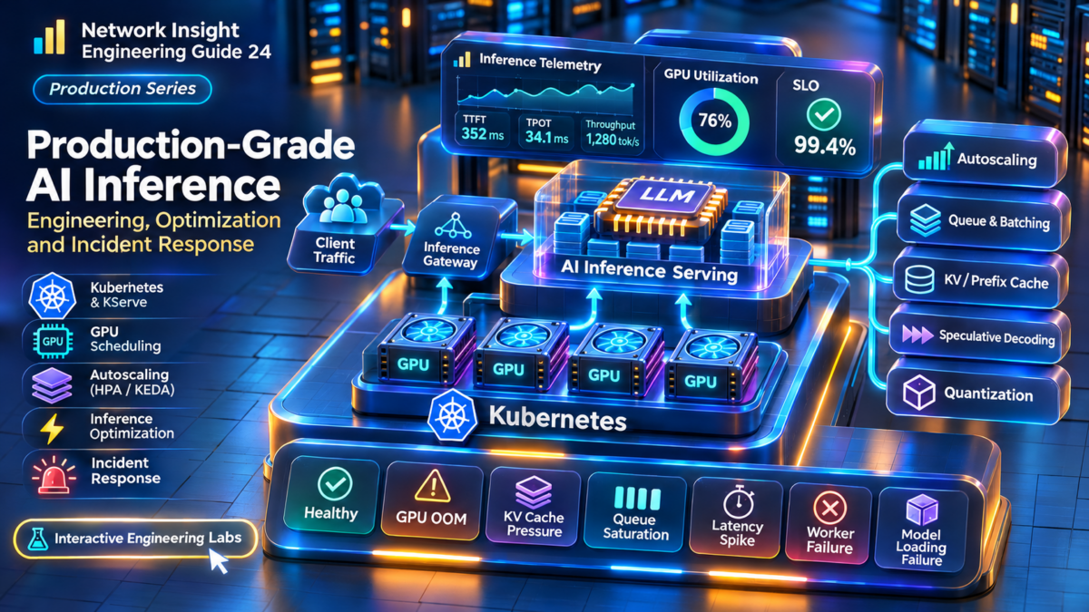
AI Model Serving Performance Engineering Explained
A production AI model-serving system must coordinate incoming requests, inference scheduling, GPU execution, memory management and streaming responses while meeting strict latency, throughput and reliability requirements.
This guide explores how LLM inference engines process prompts, how prefill and decode consume different GPU resources, how KV cache affects concurrency and how platforms such as vLLM, TensorRT-LLM, NVIDIA Triton and Kubernetes support production serving architectures.
Inside the AI Model Serving Data Path
Follow a request from the client through gateway routing, request scheduling, prefill, decode and GPU memory access. The diagram shows the major logical components rather than a fixed implementation of any single serving engine.
Investigate the Inference Execution Pipeline
The gateway accepts client requests, applies access controls and routes inference traffic toward an appropriate model-serving endpoint.
Engineering check: measure gateway latency separately from model execution time.
The Four Metrics Every Inference Engineer Must Understand
These metrics describe different aspects of the serving system. TTFT reflects initial responsiveness, TPOT captures token generation pacing, throughput measures aggregate output capacity, and concurrency describes simultaneous demand.
Six Systems That Determine Inference Performance
Inference Gateway
Routes requests, applies policy, protects endpoints and distributes demand.
Continuous Batching
Coordinates active sequences and admits work as serving capacity becomes available.
Prefill and Decode
Separates prompt processing from autoregressive token generation.
KV Cache Management
Controls attention-state memory allocation and influences concurrency limits.
GPU Serving Cluster
Provides accelerator compute, memory bandwidth and interconnect resources.
Observability and SLOs
Connects request latency, GPU utilization, queueing and failure signals.
What You Will Engineer Across Nine Sections
This guide progresses from foundational inference architecture through performance measurement, GPU memory, batching, serving engines, distributed inference, Kubernetes scaling, optimization and production troubleshooting.
Core engineering objective: Optimize the complete inference service, not GPU utilization in isolation. The best production configuration is one that meets latency and reliability targets while delivering sufficient throughput at an acceptable cost.
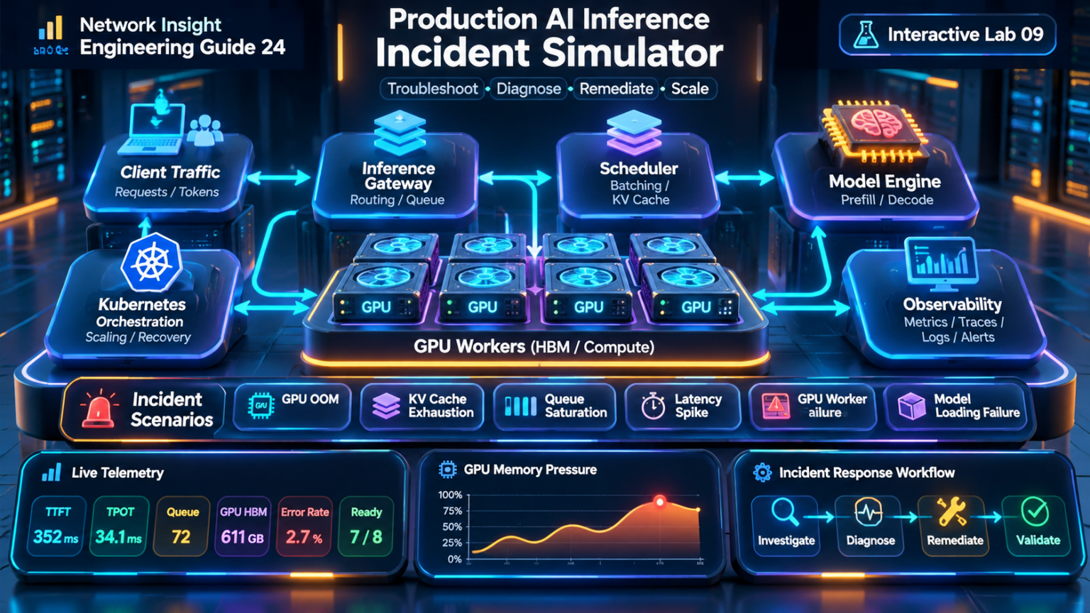
Explore the Architecture.
Engineer the Performance.
Follow the complete engineering journey through AI model serving, LLM inference performance, GPU memory, continuous batching, serving engines, distributed GPU execution, Kubernetes scaling, optimization and production troubleshooting.
Nine detailed technical sections connect the architecture of modern inference systems to the practical decisions engineers make when designing, operating and troubleshooting production AI platforms.
Engineering Guide Contents
09 TECHNICAL SECTIONSAI Model Serving Architecture Fundamentals
Production AI model serving transforms an incoming inference request into a scheduled GPU workload, executes the model, manages sequence state and returns generated output while enforcing latency, throughput and reliability objectives.
The architecture combines an API gateway, routing layer, inference scheduler, model execution engine, GPU resources, memory management and telemetry. Each component contributes to the overall response time and operating capacity of the service.
The Complete Request-to-Response Data Path
A client sends a prompt to a model-serving endpoint. The gateway authenticates and routes the request. A serving worker admits it according to available resources and scheduling policy, processes the prompt, then generates output tokens until the request finishes or terminates.
Streaming responses allow generated tokens to be delivered incrementally. This improves perceived responsiveness, but the service must still manage queueing, execution time, memory allocation and client backpressure.
Controlling Access to Model Serving Infrastructure
The gateway provides a controlled entry point for inference requests. Common responsibilities include authentication, authorization, rate limiting, request validation, model selection and routing toward available serving replicas.
Routing strategies may consider endpoint health, model availability, load, affinity and service policy. A gateway that routes only by connection count may not accurately reflect the execution cost of prompts with different token lengths.
Access Control
Authenticate clients, enforce authorization and protect serving endpoints from unauthorized traffic.
Request Routing
Direct requests toward healthy model replicas using policies appropriate for workload characteristics.
Admission Protection
Apply rate limits, quotas, deadlines and overload responses to protect downstream serving capacity.
How Requests Become GPU Execution Work
The inference scheduler determines when requests enter execution and how active sequences share accelerator resources. It must balance available KV cache memory, batch capacity, request deadlines and fairness.
Continuous batching allows the active execution batch to change between scheduling iterations, improving resource utilization compared with approaches that require all requests in a batch to finish together.
| Scheduler Function | Purpose | Engineering Risk |
|---|---|---|
| Queue management | Hold requests awaiting execution. | Excessive waiting increases TTFT. |
| Admission control | Limit active work to supported capacity. | Over-admission can exhaust memory. |
| Batch construction | Combine eligible work for execution. | Poor batching reduces efficiency. |
| Sequence management | Track active generation state. | Long-running requests may consume scarce resources. |
| Preemption or scheduling policy | Respond to capacity pressure where supported. | Recomputation or swapping can increase latency. |
Two Different Computational Phases
Prefill processes the prompt tokens and establishes the attention state used by subsequent generation. Decode then generates output tokens autoregressively, using previously cached keys and values.
The relative compute and memory requirements of each phase depend on model architecture, prompt length, batch size, context length and accelerator characteristics.
Prompt Processing
Processes the input context and creates KV state. It strongly influences initial response latency.
Token Generation
Produces successive output tokens, typically reusing the existing KV cache at each step.
Phase-Aware Scheduling
Balances prompt processing and generation to reduce interference and improve service-level performance.
Why Model Weights and KV Cache Determine Capacity
GPU memory must accommodate model weights, attention KV cache, temporary execution buffers and framework overhead. The available capacity for active sequences is therefore lower than the total advertised GPU memory.
KV cache consumption grows with sequence length and active workload size. Serving engines use different allocation and cache-management strategies to improve effective memory utilization.
Important: A GPU can have available compute capacity but insufficient memory to admit another long-context request. Production serving capacity must be evaluated across both compute and memory constraints.
Delivering Tokens While Managing Client Backpressure
Streaming APIs deliver generated output incrementally. This can reduce perceived waiting time and enables interactive applications, but it introduces connection lifecycle, cancellation and backpressure considerations.
When a client disconnects or cancels a request, the serving stack should release associated resources according to its implementation. Failure to handle cancellation efficiently can waste GPU execution and KV cache capacity.
Investigate Six Model Serving Components
Select an architecture component to inspect its role in the production inference lifecycle.
The gateway accepts inference requests, applies policy and forwards traffic toward an appropriate model-serving endpoint.
Engineering check: separate gateway latency from queueing and model execution time.
Engineering the Service Around Measurable SLOs
Reliable model serving requires observability across gateway traffic, queueing, inference execution, GPU resources and request completion. Engineers should distinguish model errors from infrastructure failures and client-side cancellations.
| Signal | What It Reveals | Operational Use |
|---|---|---|
| TTFT | Initial request responsiveness. | Identify queueing and prefill delays. |
| TPOT / ITL | Token generation pacing. | Detect decode degradation. |
| Queue depth | Waiting inference demand. | Identify saturation and admission pressure. |
| GPU memory | Memory allocation and pressure. | Investigate KV cache constraints and OOM events. |
| Tokens per second | Aggregate inference output rate. | Measure serving throughput. |
| Error and cancellation rates | Request completion reliability. | Detect overload and application failures. |
The Production Model Serving Mental Model
A production inference service is a coordinated pipeline of request management, scheduling, model execution, GPU memory allocation and response delivery.
Engineers must understand where time is spent, where requests wait, how GPU resources are shared and which component limits throughput or latency under different workload conditions.
The next section introduces the quantitative metrics used to evaluate and optimize this pipeline.
AI Model Serving Architecture Explorer
Explore how a production LLM inference request travels from a client application through an AI gateway, request scheduler, prefill execution, decode generation and GPU serving infrastructure before streaming tokens back to the client. Investigate how prompt length, output length, concurrency, GPU capacity and KV cache pressure affect the serving pipeline.
Production LLM Request-to-GPU Data Path
Select any component to inspect its role. Run a request to follow the processing sequence and observe simulated inference behavior.
Inference Workload Configuration
Inference Execution Progress
Awaiting inference request.
GPU Memory and KV Cache
Inspect a simplified GPU memory allocation for model weights, runtime overhead and active-request KV cache.
Streaming Token Output
Request Lifecycle Investigation
Inference Engineering Console
Performance Engineering Interpretation
Production AI Model Serving — Architecture Fundamentals
A production inference platform is more than a GPU running a model. It is a coordinated serving system that accepts requests, applies gateway policies, selects model replicas, schedules execution, manages accelerator memory and returns generated output to clients.
The inference gateway typically provides API authentication, routing, rate limiting, request logging and observability. It may also route traffic to different models or serving deployments according to tenant, capacity or service-level requirements.
The serving scheduler manages admission, request queues, active sequences and execution batches. Modern LLM engines may use continuous batching to improve GPU utilization while controlling latency and memory pressure.
During prefill, the model processes the input context and creates attention key/value state. During decode, the model generates additional tokens autoregressively, reusing and extending that state. Both phases execute model operations on GPU hardware; the diagram separates their logical roles rather than representing physically separate devices.
GPU memory contains model weights, KV cache allocations, temporary activations, runtime buffers and other framework allocations. Available memory often constrains the number of concurrent requests and supported context lengths.
Distributed serving can introduce communication across NVLink, NVSwitch or InfiniBand, depending on the deployment topology and parallelism strategy. The optimal architecture depends on model size, workload characteristics, hardware, cost and latency objectives.
Educational performance model. Latency and memory estimates are illustrative, not measurements of vLLM, TensorRT-LLM, NVIDIA Triton or specific GPU hardware. Real performance depends on model architecture, precision, attention implementation, hardware bandwidth, scheduling, cache reuse, networking and workload distributions.
LLM Inference Performance Metrics Explained
AI inference performance cannot be described by GPU utilization or tokens per second alone. Engineers must measure the complete request lifecycle, including queueing, prompt processing, first-token delivery, subsequent token generation and request completion.
The most important metrics include Time to First Token (TTFT), Time Per Output Token (TPOT), Inter-Token Latency (ITL), end-to-end response latency, request throughput, token throughput and concurrency.
Understanding Where Request Time Is Spent
A model-serving request may spend time waiting for admission, executing prompt prefill, generating the first output token, producing subsequent tokens and delivering the final response.
These stages have different performance characteristics. Queueing depends on demand and scheduling capacity. Prefill depends strongly on input length and model execution. Decode performance depends on output length, batching, memory access and accelerator resources.
TTFT: Measuring Initial Responsiveness
TTFT measures the elapsed time between the start of a request and the arrival or production of the first output token, depending on the measurement boundary.
It is especially important for interactive assistants, coding tools and agentic applications because users perceive the delay before the first response appears.
Engineering distinction: High TTFT does not automatically mean slow GPU compute. Queueing, request routing, long prompts and overloaded replicas can all increase the time before the first token.
Measuring the Speed of Autoregressive Generation
Inter-token latency is the elapsed time between consecutive output tokens. TPOT is commonly calculated as the average generation time per output token after the first token.
Different serving systems may expose slightly different metric definitions. Engineers should verify whether the reported value includes scheduling gaps, transport delays or other overhead.
Calculate TPOT, End-to-End Latency and Token Rate
Enter a hypothetical workload's TTFT, output-token count and average TPOT. The calculator estimates total response time and average post-first-token generation rate.
Simplified deterministic model. It assumes constant average TPOT and excludes variable network delays, pauses, batching changes and other runtime effects.
Why High Token Throughput Does Not Guarantee Low Latency
Throughput measures the amount of work completed over time. Inference systems commonly report requests per second, input tokens per second and output tokens per second.
Increasing concurrency can improve aggregate throughput by allowing the GPU to process more work, but excessive concurrency may increase queueing, memory pressure and per-request latency.
Requests per Second
Completed requests divided by elapsed measurement time.
Output Tokens per Second
Aggregate generated tokens divided by elapsed measurement time.
Active Requests
Requests simultaneously executing or resident within the serving system, according to the chosen definition.
Little's Law: For a stable system, average work in progress is approximately arrival rate multiplied by average time in the system. This helps explain why longer response times can increase the number of concurrent requests.
Why P95 and P99 Matter in Production
Average latency can hide slow requests. Percentile metrics reveal how latency is distributed across the workload.
| Metric | Meaning | Engineering Use |
|---|---|---|
| P50 | Median observed latency. | Understand typical user experience. |
| P90 | 90% of observations are at or below this value. | Monitor broader service performance. |
| P95 | 95% of observations are at or below this value. | Identify significant tail degradation. |
| P99 | 99% of observations are at or below this value. | Investigate severe tail latency and SLO risk. |
Percentiles should be calculated over a representative request population and time window. Comparing percentiles from workloads with very different prompt and output lengths can produce misleading conclusions.
Explore Three Inference Performance Profiles
Interactive chat emphasizes fast first-token delivery and smooth streaming. Long queueing delays are particularly visible to users.
Engineering focus: request routing, admission control, queue depth and decode pacing.
Turning Metrics into Service-Level Objectives
An inference SLO defines the expected service behaviour over a measurement period. Common objectives include availability, successful request completion, TTFT thresholds and token-generation latency targets.
A useful SLO must specify the measurement boundary, eligible request population, time window and threshold. Prompt length, output length and workload class may require separate SLO categories.
Measuring the Complete Inference Service
Effective inference performance engineering requires multiple complementary metrics rather than a single utilization or throughput number.
TTFT measures initial responsiveness, TPOT and ITL describe generation pacing, throughput measures completed work, concurrency reflects demand and percentile distributions expose tail latency.
The next section investigates the GPU memory architecture that often determines the maximum concurrency and context capacity of an LLM serving system.
Inference Latency & Throughput Analyzer
Investigate the performance of a production LLM serving system. Adjust prompt size, generated tokens, arrival rate, batching, GPU capacity and serving efficiency to understand the relationship between time to first token, inter-token latency, end-to-end response time and aggregate throughput.
LLM Request Latency Timeline
Each phase contributes to user-visible response latency. The timeline below shows the modeled request's queueing, prefill, first-token decode and remaining output-token generation.
Inference Performance Controls
Latency–Throughput Operating Curve
Explore how offered load approaches modeled service capacity. As utilization increases, queueing delay rises sharply; sustained overload cannot be served without a growing backlog or admission control.
Estimated GPU serving utilization: —
Service-Level Objectives and Capacity
Engineering Findings
Inference Metrics and Diagnostic Console
Performance Metrics Reference
| Metric | Definition |
|---|---|
| TTFT | Request arrival to first output token |
| TPOT | Mean time per output token after the first |
| ITL | Time between successive output tokens |
| E2E latency | Request arrival to final response completion |
| Output TPS | Aggregate generated output tokens per second |
| Concurrency | Number of requests in service or waiting |
| Utilization | Fraction of modeled serving capacity consumed |
TPOT and ITL are closely related but not necessarily identical in real deployments: ITL is a distribution of token-to-token intervals, while TPOT is typically reported as a per-request average.
Production LLM Performance Engineering — Interpretation
TTFT is especially important for interactive assistants, chat interfaces and streaming APIs. It includes gateway overhead, queueing, prompt prefill and first-token generation. Long prompts and heavily loaded serving engines can increase TTFT substantially.
TPOT and ITL characterize the cadence of autoregressive decoding. Token generation may be constrained by model memory bandwidth, GPU compute, attention operations, active batch size and scheduling interference.
Throughput must be evaluated alongside latency. Maximizing aggregate tokens per second may increase per-request latency, particularly under heavy batching or sustained contention. The best operating point depends on the workload's SLOs.
Queueing and saturation require explicit admission control, capacity planning and autoscaling. A serving system that receives more work than it can sustainably process will accumulate a backlog unless requests are throttled, rejected or diverted.
Observability should separate gateway latency, queue time, prefill duration, decode timing, token throughput, GPU memory utilization and application-visible tail latency. A single average response-time metric is insufficient for production diagnosis.
All estimates in this laboratory are synthetic and deterministic. The service model assumes homogeneous requests, a simplified batching benefit and a single aggregate capacity pool. It does not represent measured performance of any particular GPU, model, vLLM, TensorRT-LLM or Triton deployment. The operating curve uses a finite illustrative queue-delay approximation; overload is flagged rather than presented as a stable queueing state.
GPU Memory and KV Cache Architecture Explained
GPU memory is one of the most important capacity constraints in production LLM inference. Model weights, attention KV cache, temporary execution buffers and runtime overhead must coexist within the available accelerator memory budget.
As context lengths and active sequence counts increase, KV cache allocation becomes a major determinant of concurrency, latency and service reliability. Techniques such as PagedAttention, prefix caching and memory-aware scheduling help serving engines use memory more effectively.
The Four Major Consumers of GPU Memory
A model-serving engine must reserve memory for model parameters, attention state, temporary computation and runtime operations. The amount available for KV cache depends on model size, precision, deployment topology and serving-engine configuration.
Model Weights
Persistent model parameters loaded into accelerator memory for inference execution.
KV Cache
Stored attention keys and values used to avoid recomputing prior sequence state during generation.
Runtime and Buffers
Temporary activations, execution workspaces, communication buffers and framework allocations.
Engineering principle: Available GPU memory is not equivalent to available KV cache capacity. The serving engine must account for all memory consumers and maintain operational headroom.
How the KV Cache Supports Autoregressive Generation
Transformer attention uses query, key and value representations. During autoregressive inference, the keys and values from previous tokens can be retained so that each new decode step does not need to recompute the full historical attention state.
KV cache memory generally grows with the number of retained tokens, attention layers, KV heads and head dimensions. Grouped-query and multi-query attention can reduce cache requirements compared with conventional multi-head attention.
Estimating Memory Required Per Token
For a conventional transformer with a uniform attention configuration, an approximate KV cache capacity formula is:
The formula must be adjusted for models with non-uniform attention layers, sliding-window attention, hybrid architectures, quantized KV cache formats or other specialized attention mechanisms.
Estimate KV Cache Capacity and Sequence Concurrency
Configure a simplified GPU memory budget and KV cache requirement. The calculator estimates remaining memory and how many equal-length sequences could fit within the KV cache allocation.
Capacity is a theoretical estimate. Actual concurrency depends on scheduling, block allocation, token distributions and serving-engine behaviour.
Separating Logical KV Blocks from Physical Memory
PagedAttention uses block-based KV cache management, allowing logical token blocks to map to physical memory blocks without requiring each sequence to occupy one contiguous memory region.
This approach can reduce allocation waste and improve memory sharing and reuse. However, block rounding, fragmentation within the final block and runtime metadata still contribute to memory overhead.
| Memory Strategy | Architectural Behaviour | Engineering Consideration |
|---|---|---|
| Contiguous allocation | Reserve a continuous region for sequence KV state. | May create allocation waste and capacity constraints. |
| Paged KV allocation | Map logical sequence blocks to physical cache blocks. | Improves allocation flexibility but requires block management. |
| Prefix caching | Reuse eligible previously computed KV blocks for matching prefixes. | Requires cache validity, matching rules and eviction policies. |
| Preemption | Temporarily suspend or reschedule sequences under resource pressure. | Can introduce recomputation or data movement overhead. |
Reducing Repeated Prompt Computation
Many inference requests share common system prompts, instructions or retrieved context. Prefix caching can reuse previously computed KV state when the serving engine determines that the prefix is eligible and matches the new request.
Cache effectiveness depends on workload similarity, cache retention, memory availability, model configuration and the serving engine's matching and isolation rules.
Security consideration: Prefix caching must respect tenant isolation and data access boundaries. Shared cache resources should never allow one tenant to retrieve another tenant's protected prompt content.
Investigate Four GPU Memory Conditions
Active sequences fit within the available KV cache budget. The scheduler can admit new requests while maintaining operational memory headroom.
Engineering check: monitor allocated cache blocks, free capacity and active sequence count.
Diagnosing GPU Memory and KV Cache Failures
Memory-related inference failures may appear as rejected requests, sudden TTFT increases, reduced concurrency, repeated preemption, allocation errors or GPU out-of-memory events.
| Symptom | Potential Cause | Investigation |
|---|---|---|
| High TTFT | Requests waiting for KV capacity. | Inspect queue depth and cache utilization. |
| Reduced concurrency | Long contexts consume more KV memory. | Compare sequence lengths and memory allocation. |
| GPU OOM | Memory allocations exceed available capacity. | Inspect weights, runtime buffers and KV budget. |
| High recomputation | Preemption or cache eviction. | Review scheduler and cache-management telemetry. |
| Low prefix cache hit rate | Insufficient matching prefixes or frequent eviction. | Inspect workload similarity and cache retention. |
GPU Memory Is a First-Class Serving Resource
Production LLM inference capacity depends on both accelerator compute and the memory required to keep model weights, runtime buffers and active sequence state resident.
KV cache management, PagedAttention, prefix caching and memory-aware scheduling are essential techniques for improving effective concurrency and reducing unnecessary memory waste.
The next section explores how continuous batching and request scheduling coordinate these resources under changing inference demand.
GPU Memory & KV Cache Simulator
Investigate how model weights, runtime allocations, active context lengths, concurrent requests and attention KV cache compete for GPU high-bandwidth memory. Explore how block-based KV allocation changes internal fragmentation, why admission control matters, and how GPU memory pressure affects production LLM inference.
GPU HBM Allocation Explorer
The bar shows aggregate modeled memory allocation across the configured GPU group. In a real deployment, memory placement and per-GPU limits must also be checked independently.
Paged KV Cache Block Map
Each tile represents a logical cache block in a sampled allocation pool. Gold tiles contain active KV data, purple tiles represent partially filled allocations, and dark tiles are free.
GPU and Model Configuration
Memory Capacity and Admission Control
Aggregate GPU HBM pressure
Awaiting calculation.
KV Cache Architecture Analysis
GPU Memory Diagnostic Console
Production Troubleshooting Checklist
GPU Memory and KV Cache — Engineering Fundamentals
LLM inference requires persistent model weights, temporary runtime allocations and attention key/value state. KV cache capacity is influenced by model layers, KV heads, head dimension, cache precision, active sequence lengths and request concurrency.
For a conventional transformer KV representation, approximate cache bytes per token are 2 × layers × KV heads × head dimension × bytes per element. The factor of two accounts for keys and values. Grouped-query attention reduces KV head count relative to attention query heads, which can substantially reduce cache memory requirements.
Paged KV allocation divides attention cache storage into blocks and allocates them as sequences grow. It can reduce wasted reservation and simplify block management, but does not eliminate internal fragmentation, memory bandwidth constraints or all allocator overhead. Prefix sharing, sliding-window attention and specialized cache compression can change the memory model further.
Tensor parallelism may shard model weights and KV cache across GPUs, depending on the engine and parallelism configuration. Aggregate free memory alone does not guarantee admission: a single GPU can exhaust its local memory while others retain capacity.
Real production memory engineering must consider GPU hardware capacity, model loading formats, quantization metadata, attention kernels, CUDA graphs, activation peaks, memory fragmentation and engine-specific allocation policies.
Educational model only. All GPUs are assumed to provide 80 GB of HBM, with idealized balanced tensor-parallel sharding and synthetic runtime overhead. Large MoE memory is represented by an illustrative parameter-residency profile. This widget does not measure actual GPU memory or implement NVIDIA PagedAttention kernels.
Continuous Batching and Request Scheduling Explained
Continuous batching allows LLM serving engines to change the set of active requests between execution iterations, admitting new work as resources become available rather than waiting for an entire fixed batch to finish.
The scheduler must coordinate prefill execution, decode iterations, KV cache capacity, request admission, fairness and latency objectives. Its decisions directly affect TTFT, TPOT, throughput and service reliability.
How the Scheduler Coordinates GPU Execution
Incoming inference requests enter a waiting queue. The scheduler determines which requests can execute based on token budgets, available KV cache capacity, model configuration and serving-engine policies.
Once admitted, a request performs prompt prefill and enters token generation. At scheduling boundaries, the engine may admit additional requests, continue existing sequences or preempt work when capacity becomes constrained.
Why Iteration-Level Scheduling Matters
In a static batch, requests may remain grouped for the duration of execution. Shorter requests can leave compute capacity underused while longer requests continue.
Continuous batching allows completed sequences to leave and new eligible sequences to enter at scheduling boundaries. This can improve throughput and GPU efficiency, although admission and batching decisions still affect individual request latency.
Fixed Request Group
A batch is assembled before execution and may not admit replacements until the batch completes.
Dynamic Active Set
Requests can join or leave between iterations, subject to available capacity and engine policy.
Throughput Versus Latency
Larger active batches can improve aggregate throughput while increasing per-request latency under some workloads.
Scheduling Two Different Workload Phases
Prefill processes prompt tokens and often benefits from substantial parallel computation. Decode produces tokens incrementally and may be sensitive to memory bandwidth, batching and scheduling delays.
A large prefill workload can delay decode iterations when both phases share execution resources. Chunked prefill, scheduling priorities and disaggregated prefill/decode architectures are techniques used to manage this interference.
Production principle: Improving aggregate GPU utilization is not sufficient if interactive users experience unacceptable first-token or inter-token latency.
Run a Simplified Continuous-Batching Engine
Add requests, advance execution iterations and observe how the scheduler admits queued work. Each request requires one prefill iteration followed by a configurable number of decode iterations.
Waiting Queue
Active GPU Batch — Maximum 3
Completed Requests
Scheduler Event Log
Educational simulator: fixed three-request active capacity, one prefill step and 2–5 decode steps per request. It does not model GPU kernel timing, real KV cache allocation, chunked prefill or preemption.
Why Not Every Request Can Execute Immediately
Admission decisions must account for more than the number of requests. Prompt length, expected output length, KV cache capacity, active sequence count and configured token budgets influence whether new work can be scheduled.
| Constraint | Scheduling Impact | Operational Signal |
|---|---|---|
| Maximum active sequences | Limits concurrent requests. | Running request count |
| Token budget | Limits tokens scheduled in an iteration. | Scheduled tokens per step |
| KV cache capacity | Limits resident attention state. | Allocated and free KV blocks |
| Request deadlines | May influence scheduling priority. | Deadline misses and queue delay |
| Fairness policy | Controls how competing requests receive capacity. | Per-class waiting time |
Preventing Starvation and Excessive Tail Latency
First-in-first-out scheduling is simple but does not account for request size or priority. Alternative policies may consider waiting time, expected workload, service class or latency deadlines.
Fairness matters in shared inference platforms where long-context requests, short interactive requests and background jobs compete for the same GPU resources. Strict prioritization can improve one class of service while starving another.
What Happens When the Active Batch Exceeds Memory Capacity?
When KV cache capacity becomes constrained, the scheduler may delay new admissions, preempt active sequences or use supported memory-management techniques. Some implementations recompute discarded state when a sequence resumes.
Preemption can preserve service availability under overload, but repeated preemption or recomputation increases latency and wastes accelerator work. Engineers should correlate preemption events with KV cache utilization and request-length distributions.
Designing a Scheduler for Real Workload Behaviour
| Observed Symptom | Possible Cause | Engineering Response |
|---|---|---|
| High TTFT | Queueing or delayed prefill. | Inspect admission capacity and prefill scheduling. |
| High TPOT | Decode interference or overloaded batches. | Inspect iteration latency and active batch size. |
| Low throughput | Underfilled batches or inefficient execution. | Measure batch occupancy and GPU utilization. |
| Frequent preemption | KV cache pressure. | Review memory budget and sequence lengths. |
| Unfair latency | Priority or scheduling imbalance. | Compare queueing by workload class. |
The Scheduler Is the Control Plane of LLM Execution
Continuous batching improves resource sharing by allowing the active request set to change at execution boundaries. Its effectiveness depends on admission policy, token budgets, memory availability and workload characteristics.
The next section compares the serving engines that implement these scheduling and execution capabilities in production AI platforms.
Continuous Batching & Request Scheduler
Operate a simplified LLM inference scheduler. Generate requests, inspect the waiting queue, observe prefill and decode execution, and compare continuous batching with static batching. Experiment with GPU execution slots, KV token budgets, priority scheduling and admission control.
Live Inference Scheduling Pipeline
Requests move from the waiting queue into prefill and decode execution. Each scheduler tick advances the active batch. Gold-edged requests are high priority.
KV Token Budget Utilization
0 / 0 KV tokens allocated.
Scheduler Engineering Controls
For visibility, each simulated decode tick represents multiple output tokens. The lab focuses on scheduling decisions, not physical token timing.
Scheduler Diagnostics
Live Engineering Assessment
Continuous Batching — Engineering Fundamentals
Static batching groups requests into a fixed execution cohort. Depending on the implementation, newly arriving requests may wait until that cohort finishes. Continuous batching allows requests to enter and leave execution as scheduler iterations progress, improving accelerator occupancy when sequence lengths vary.
Prefill processes the input prompt and establishes the initial attention KV state. Decode generates subsequent tokens autoregressively. Because prefill can be compute-intensive while decode may be constrained by memory movement, mixing these phases can create interference and latency variability.
Production schedulers also consider token budgets, memory capacity, fairness, priority, preemption and maximum running sequences. A request may be queued even when a nominal execution slot is free if sufficient KV memory is unavailable.
Priority scheduling can reduce latency for important workloads but may starve lower-priority requests without aging or fairness controls. Real serving systems may also use chunked prefill, prefix caching, disaggregated prefill/decode, speculative decoding and engine-specific scheduling policies.
Educational discrete-event simulator. GPU slots, prefill work, decode work and KV reservations are simplified abstractions. The lab does not run real model kernels or reproduce an exact vLLM, Triton or TensorRT-LLM implementation.
vLLM, TensorRT-LLM and NVIDIA Triton Architecture Explained
Production model serving requires a runtime capable of loading models, managing GPU execution, scheduling inference requests and exposing reliable inference endpoints.
vLLM, NVIDIA TensorRT-LLM and NVIDIA Triton Inference Server address overlapping but different layers of the serving architecture. Understanding these distinctions helps engineers select the right runtime and deployment model.
Understanding the Layers of an Inference Platform
An inference platform commonly includes an API entry point, model-serving runtime, scheduling and execution components, accelerator libraries and GPU hardware.
These layers are not always separate processes. Some frameworks integrate API serving, scheduling and model execution, while others use a serving server that delegates execution to specialized backends.
High-Throughput LLM Serving with Efficient Scheduling
vLLM is an LLM inference and serving framework that integrates request scheduling, model execution and KV cache management. It is commonly used to expose API-compatible model endpoints.
Its architecture emphasizes efficient memory management and dynamic request execution. PagedAttention and continuous batching are important concepts associated with vLLM, although supported execution features vary by release, hardware and model.
Continuous Batching
Coordinates active inference sequences and admits new work as execution resources become available.
Paged KV Management
Uses block-based attention cache allocation to improve memory flexibility.
Model Serving APIs
Supports API-based inference deployments with model and runtime configuration.
Optimized LLM Execution on NVIDIA Accelerators
TensorRT-LLM provides NVIDIA-oriented LLM inference optimizations and runtime capabilities. Its execution architecture can use optimized kernels, quantization, batching and distributed inference techniques where supported.
Engineers must consider GPU architecture, supported model features, precision, execution configuration and deployment integration. The best performance configuration depends on the actual workload and model.
Engineering distinction: TensorRT-LLM is not simply a substitute name for Triton. TensorRT-LLM provides LLM execution capabilities, while Triton provides a broader model-serving server that can integrate supported execution backends.
Serving Models Through a Multi-Backend Platform
NVIDIA Triton Inference Server provides a serving environment for supported model formats and execution backends. It exposes inference APIs and supports model management, scheduling capabilities and deployment integrations.
Triton can serve different model workloads through compatible backends. For LLM deployments, TensorRT-LLM may be integrated through its supported backend configuration.
Inference Endpoints
Exposes serving interfaces for clients and upstream applications.
Execution Integration
Connects supported model formats and execution backends to the serving platform.
Model Management
Provides model lifecycle and operational capabilities depending on configuration.
Understanding the Architectural Differences
| Dimension | vLLM | TensorRT-LLM | NVIDIA Triton |
|---|---|---|---|
| Primary role | LLM inference and serving framework. | Optimized LLM execution framework/runtime. | General-purpose inference serving server. |
| Request scheduling | Integrated LLM scheduling. | Supported scheduling and batching capabilities. | Scheduling depends on model/backend configuration. |
| KV cache | Block-based KV management. | Optimized KV management capabilities. | Managed primarily by the selected LLM backend. |
| Deployment | Standalone or integrated LLM serving. | LLM runtime and backend integrations. | Serving server with supported backends. |
| Engineering focus | LLM serving efficiency and flexibility. | NVIDIA accelerator execution optimization. | Model-serving operations and backend integration. |
Inspect Each Serving Architecture
Select a serving technology to explore its architectural responsibilities and operational considerations.
vLLM integrates LLM request scheduling, KV cache management, model execution and API serving capabilities.
Engineering check: evaluate TTFT, TPOT, throughput, KV cache usage and model compatibility.
Designing the Serving Platform Around Workload Requirements
A production deployment may run inference workers behind an API gateway, load balancer or Kubernetes service. Replicas can be scaled to meet workload demand, subject to GPU availability, model-loading time and scheduling constraints.
Diagnosing Model Serving Runtime Problems
| Symptom | Potential Cause | Investigation |
|---|---|---|
| High TTFT | Queueing, prefill overhead or model initialization. | Inspect request timing and scheduler metrics. |
| Low throughput | Small batches or inefficient execution configuration. | Compare batch occupancy and GPU telemetry. |
| GPU OOM | Weights, KV cache or runtime buffers exceed capacity. | Inspect GPU memory allocation and engine configuration. |
| Model load failure | Unsupported model, incompatible configuration or missing artifacts. | Review backend logs, model files and compatibility. |
| Replica instability | Resource exhaustion or deployment lifecycle issues. | Inspect readiness, health checks and container logs. |
Selecting the Correct Serving Architecture
vLLM, TensorRT-LLM and NVIDIA Triton occupy related but distinct positions in the AI model-serving ecosystem.
Serving-engine selection should be based on model compatibility, hardware, latency requirements, throughput, operational integration and measurable production performance.
The next section explores how inference execution scales across multiple GPUs and servers using tensor parallelism, pipeline parallelism and distributed communication.
vLLM, TensorRT-LLM and NVIDIA Triton Architecture Explained
Production model serving requires a runtime capable of loading models, managing GPU execution, scheduling inference requests and exposing reliable inference endpoints.
vLLM, NVIDIA TensorRT-LLM and NVIDIA Triton Inference Server address overlapping but different layers of the serving architecture. Understanding these distinctions helps engineers select the right runtime and deployment model.
Understanding the Layers of an Inference Platform
An inference platform commonly includes an API entry point, model-serving runtime, scheduling and execution components, accelerator libraries and GPU hardware.
These layers are not always separate processes. Some frameworks integrate API serving, scheduling and model execution, while others use a serving server that delegates execution to specialized backends.
High-Throughput LLM Serving with Efficient Scheduling
vLLM is an LLM inference and serving framework that integrates request scheduling, model execution and KV cache management. It is commonly used to expose API-compatible model endpoints.
Its architecture emphasizes efficient memory management and dynamic request execution. PagedAttention and continuous batching are important concepts associated with vLLM, although supported execution features vary by release, hardware and model.
Continuous Batching
Coordinates active inference sequences and admits new work as execution resources become available.
Paged KV Management
Uses block-based attention cache allocation to improve memory flexibility.
Model Serving APIs
Supports API-based inference deployments with model and runtime configuration.
Optimized LLM Execution on NVIDIA Accelerators
TensorRT-LLM provides NVIDIA-oriented LLM inference optimizations and runtime capabilities. Its execution architecture can use optimized kernels, quantization, batching and distributed inference techniques where supported.
Engineers must consider GPU architecture, supported model features, precision, execution configuration and deployment integration. The best performance configuration depends on the actual workload and model.
Engineering distinction: TensorRT-LLM is not simply a substitute name for Triton. TensorRT-LLM provides LLM execution capabilities, while Triton provides a broader model-serving server that can integrate supported execution backends.
Serving Models Through a Multi-Backend Platform
NVIDIA Triton Inference Server provides a serving environment for supported model formats and execution backends. It exposes inference APIs and supports model management, scheduling capabilities and deployment integrations.
Triton can serve different model workloads through compatible backends. For LLM deployments, TensorRT-LLM may be integrated through its supported backend configuration.
Inference Endpoints
Exposes serving interfaces for clients and upstream applications.
Execution Integration
Connects supported model formats and execution backends to the serving platform.
Model Management
Provides model lifecycle and operational capabilities depending on configuration.
Understanding the Architectural Differences
| Dimension | vLLM | TensorRT-LLM | NVIDIA Triton |
|---|---|---|---|
| Primary role | LLM inference and serving framework. | Optimized LLM execution framework/runtime. | General-purpose inference serving server. |
| Request scheduling | Integrated LLM scheduling. | Supported scheduling and batching capabilities. | Scheduling depends on model/backend configuration. |
| KV cache | Block-based KV management. | Optimized KV management capabilities. | Managed primarily by the selected LLM backend. |
| Deployment | Standalone or integrated LLM serving. | LLM runtime and backend integrations. | Serving server with supported backends. |
| Engineering focus | LLM serving efficiency and flexibility. | NVIDIA accelerator execution optimization. | Model-serving operations and backend integration. |
Inspect Each Serving Architecture
Select a serving technology to explore its architectural responsibilities and operational considerations.
vLLM integrates LLM request scheduling, KV cache management, model execution and API serving capabilities.
Engineering check: evaluate TTFT, TPOT, throughput, KV cache usage and model compatibility.
Designing the Serving Platform Around Workload Requirements
A production deployment may run inference workers behind an API gateway, load balancer or Kubernetes service. Replicas can be scaled to meet workload demand, subject to GPU availability, model-loading time and scheduling constraints.
Diagnosing Model Serving Runtime Problems
| Symptom | Potential Cause | Investigation |
|---|---|---|
| High TTFT | Queueing, prefill overhead or model initialization. | Inspect request timing and scheduler metrics. |
| Low throughput | Small batches or inefficient execution configuration. | Compare batch occupancy and GPU telemetry. |
| GPU OOM | Weights, KV cache or runtime buffers exceed capacity. | Inspect GPU memory allocation and engine configuration. |
| Model load failure | Unsupported model, incompatible configuration or missing artifacts. | Review backend logs, model files and compatibility. |
| Replica instability | Resource exhaustion or deployment lifecycle issues. | Inspect readiness, health checks and container logs. |
Selecting the Correct Serving Architecture
vLLM, TensorRT-LLM and NVIDIA Triton occupy related but distinct positions in the AI model-serving ecosystem.
Serving-engine selection should be based on model compatibility, hardware, latency requirements, throughput, operational integration and measurable production performance.
The next section explores how inference execution scales across multiple GPUs and servers using tensor parallelism, pipeline parallelism and distributed communication.
Distributed Inference and GPU Parallelism Explained
Large AI models frequently require more memory or compute capacity than a single accelerator can provide. Distributed inference partitions model execution across multiple GPUs and, when necessary, multiple servers.
Engineers must understand tensor parallelism, pipeline parallelism, expert parallelism, GPU interconnects and distributed communication to design inference platforms that scale without introducing excessive latency or network overhead.
Scaling Model Execution Beyond a Single GPU
Distributed inference uses multiple accelerators to execute one model or serve a collection of model replicas. Model-parallel techniques partition work across GPUs, while data-parallel serving typically places independent model replicas on separate GPU groups.
The performance of distributed execution depends on how frequently GPUs exchange data, the volume of communication and the bandwidth and latency of the underlying interconnect.
Partitioning Model Computation Across GPUs
Tensor parallelism partitions selected tensor operations across multiple accelerators. For example, portions of matrix multiplication or attention computation may execute on different GPUs.
GPUs often need to exchange partial results using collective communication operations. The cost of these operations depends on tensor size, parallel group size, network bandwidth and communication latency.
Tensor Shards
Distribute supported model computations and parameter partitions across GPUs.
Collective Operations
Exchange or combine partial results through operations such as all-reduce and all-gather.
Communication Overhead
Increasing tensor-parallel degree can reduce per-GPU model memory while increasing coordination costs.
Distributing Transformer Layers Across Stages
Pipeline parallelism assigns groups of model layers to different GPUs or GPU groups. Activations move between pipeline stages as requests progress through the model.
Pipeline execution can reduce per-GPU weight memory, but stage imbalance and pipeline bubbles may reduce utilization. Serving engines may use microbatching and scheduling techniques to improve stage occupancy.
Scaling Mixture-of-Experts Model Execution
Mixture-of-Experts models contain multiple expert networks, with routing logic selecting a subset of experts for each token. Expert parallelism distributes experts across accelerators.
Tokens may need to move between GPUs hosting selected experts. This introduces all-to-all communication patterns and can create load imbalance when some experts receive more tokens than others.
Engineering principle: Expert-parallel performance depends not only on network bandwidth but also on token routing distribution, expert placement, collective communication efficiency and scheduling behaviour.
Compare Distributed Inference Strategies
Select a parallelism strategy to inspect its model partitioning, communication pattern and operational considerations.
Model tensor operations are partitioned across GPUs. Partial results may require collective communication during execution.
Engineering check: inspect collective latency, GPU synchronization and per-GPU memory usage.
NVLink, NVSwitch, InfiniBand and NCCL
Distributed inference performance depends on the communication path between GPUs. Intra-node GPU connectivity may use NVLink and NVSwitch where supported, while multi-node clusters often rely on high-performance Ethernet or InfiniBand networking.
NVIDIA Collective Communications Library (NCCL) provides collective communication operations commonly used in distributed GPU workloads. Its performance depends on topology, transport configuration and communication patterns.
| Technology | Architectural Role | Engineering Consideration |
|---|---|---|
| NVLink | High-bandwidth GPU connectivity on supported systems. | GPU generation, topology and link bandwidth. |
| NVSwitch | Switching fabric connecting GPUs in supported platforms. | Fabric topology and collective communication. |
| InfiniBand | High-performance inter-node network transport. | RDMA, congestion, routing and fabric health. |
| NCCL | GPU collective communication library. | Collective algorithms, transport and synchronization. |
Estimate Model Weight Memory Across Tensor-Parallel GPUs
Enter model parameter count, weight precision and tensor-parallel degree. The calculator estimates the idealized weight-memory allocation per GPU, excluding KV cache, activations and runtime overhead.
Simplified capacity model. Quantization metadata, replicated parameters, uneven partitioning, KV cache, runtime buffers and communication overhead are excluded. It does not predict inference speed.
Diagnosing Distributed Inference Bottlenecks
| Symptom | Potential Cause | Investigation |
|---|---|---|
| High inter-token latency | Collective communication or synchronization overhead. | Profile GPU kernels and communication operations. |
| Low GPU utilization | Pipeline bubbles or communication stalls. | Inspect stage timing and GPU activity. |
| Uneven expert utilization | MoE routing imbalance. | Measure expert token distribution. |
| Multi-node slowdown | Network latency, congestion or transport configuration. | Inspect fabric telemetry and collective benchmarks. |
| GPU OOM | Uneven memory partitioning or KV cache pressure. | Compare memory allocation across GPU ranks. |
Parallelism Is a Compute and Networking Design Decision
Distributed inference is not simply a matter of adding GPUs. It requires selecting model partitioning strategies and communication topologies that match the model architecture and workload.
Tensor parallelism distributes tensor operations, pipeline parallelism distributes layers, expert parallelism distributes MoE experts and data-parallel serving distributes independent model replicas.
The next section investigates how Kubernetes schedules, deploys and scales GPU inference workloads in production environments.
Distributed Inference Topology Designer
Design and investigate distributed LLM inference across multiple GPU servers. Compare tensor parallelism, pipeline parallelism and expert parallelism. Explore GPU placement, memory distribution, NVLink/NVSwitch communication, InfiniBand inter-node transport and failure-domain considerations.
Multi-Node GPU Serving Fabric
Inspect how GPUs are grouped into model execution partitions. Cyan links represent active modeled communication paths. A red link indicates an injected fabric failure.
GPU Memory Allocation
Awaiting configuration.
Distributed Inference Controls
The visual topology displays up to four servers with the configured GPU count per server.
Parallelism Strategy Assessment
Interconnect and Failure-Domain Analysis
Distributed Inference Diagnostics
Production Engineering Checklist
Distributed Inference — Engineering Fundamentals
Tensor parallelism partitions tensor operations across GPUs. It can reduce per-device model weight residency but introduces communication for distributed matrix operations and collective synchronization.
Pipeline parallelism places different model stages on different devices or groups. It reduces per-device layer residency but introduces activation transfers and potential pipeline bubbles.
Expert parallelism distributes experts in mixture-of-experts models. Token dispatch and expert output collection can create all-to-all communication and network sensitivity.
NVLink and NVSwitch provide high-bandwidth communication within supported GPU systems, while InfiniBand and RoCE-based networks connect accelerator nodes across the cluster. Actual topology and bandwidth depend on the hardware generation.
Distributed inference capacity depends on more than total GPU count. Communication patterns, parallel group placement, model partitioning, KV cache layout, batching, context length and fault tolerance all influence production performance.
Educational topology model only. Each GPU is assumed to provide 80 GB of HBM. Communication and latency indices are synthetic, dimensionless values and are not hardware measurements. The memory model assumes idealized balanced placement.
Kubernetes AI Inference Scaling Explained
Kubernetes provides the orchestration layer for deploying, scheduling and operating AI inference workloads across GPU-enabled infrastructure. However, scaling an inference service requires more than increasing the number of Pods.
Engineers must coordinate GPU allocation, model-loading time, serving-engine readiness, request routing, autoscaling metrics, queue depth and available accelerator capacity to maintain predictable inference latency under changing demand.
How Requests Reach GPU-Backed Model Servers
A typical Kubernetes inference architecture places an API gateway or inference-aware routing layer in front of model-serving Pods. The serving Pods run frameworks such as vLLM or supported TensorRT-LLM-based deployments.
Kubernetes schedules Pods onto eligible GPU nodes using resource requests, node placement constraints and device-plugin-advertised resources. An autoscaling controller adjusts replica counts using supported metrics, while cluster-level capacity management provides additional nodes when necessary.
How Kubernetes Allocates Accelerator Resources
Kubernetes relies on device plugins or equivalent supported resource-management integrations to advertise GPU resources to the scheduler. GPU workloads request those resources through Pod specifications.
The NVIDIA GPU Operator can automate deployment and management of supported GPU software components, including drivers, device plugins and monitoring components, depending on platform configuration.
GPU Device Plugin
Advertises supported accelerator resources to Kubernetes.
NVIDIA GPU Operator
Helps manage the GPU software stack across supported Kubernetes environments.
GPU Node Scheduling
Uses resource availability, placement constraints and scheduling policies to place Pods.
Model Serving as a Kubernetes-Native Service
KServe provides Kubernetes-oriented model-serving abstractions and deployment capabilities. Supported serving modes and integrations can simplify the management of inference endpoints.
The runtime selection, deployment mode and model requirements determine how KServe interacts with model servers, autoscaling and networking components. Engineers should validate the exact KServe version and runtime integration rather than assuming every engine supports the same capabilities.
Architecture distinction: KServe manages model-serving deployment abstractions, while the selected inference runtime performs model execution. Kubernetes supplies scheduling and infrastructure orchestration.
HPA, KEDA and Queue-Aware Scaling
CPU utilization is often a poor standalone signal for GPU inference capacity. More relevant signals may include request arrival rate, queue depth, active sequences, TTFT, token throughput and GPU or KV cache pressure.
Horizontal Pod Autoscaler can scale using supported resource, custom or external metrics. KEDA can provide event-driven scaling using supported scalers and metrics adapters.
| Scaling Signal | Benefit | Limitation |
|---|---|---|
| CPU utilization | Simple infrastructure metric. | May not reflect GPU inference saturation. |
| Request queue depth | Responds to pending work. | Requires appropriate queue visibility and tuning. |
| Active sequences | Reflects concurrent inference execution. | Sequence lengths and resource requirements vary. |
| TTFT / latency | Connects scaling to user experience. | Can react after performance degradation begins. |
| GPU / KV utilization | Provides resource pressure signals. | High utilization is not always equivalent to overload. |
Estimate GPU Serving Replicas for Request Demand
Enter the expected request arrival rate, measured sustainable throughput per replica and target utilization. The calculator estimates the required replica count under a simplified steady-state capacity model.
Illustrative steady-state calculation. Real inference capacity depends on prompt length, output length, model, batching, GPU memory, SLO targets and traffic variability. This is not a prediction of autoscaler behaviour.
Why GPU Inference Replicas Cannot Always Scale Instantly
A new inference Pod may need to wait for GPU node capacity, pull a container image, access model artifacts, initialize the serving runtime, load weights into GPU memory and complete readiness checks.
These steps can introduce substantial startup delays. Production scaling strategies may require pre-provisioned GPU capacity, warm replicas, cached model artifacts and carefully designed readiness gates.
Compare Four Production Scaling Scenarios
Demand remains relatively stable. The platform can maintain a suitable number of warm serving replicas with predictable request distribution.
Engineering check: monitor replica utilization, TTFT, queue depth and capacity headroom.
Diagnosing Kubernetes Inference Scaling Failures
| Symptom | Potential Cause | Investigation |
|---|---|---|
| Pending GPU Pods | Insufficient accelerator resources or placement constraints. | Inspect scheduler events, GPU allocatable resources and node labels. |
| Slow scale-out | Model loading or GPU node provisioning delays. | Measure Pod startup, model initialization and readiness duration. |
| High TTFT during bursts | Serving capacity cannot absorb incoming demand. | Correlate arrival rate, queue depth and available replicas. |
| Autoscaling oscillation | Unstable metrics or poorly tuned scaling policies. | Review stabilization windows and scaling thresholds. |
| GPU underutilization | Low request volume, poor batching or uneven routing. | Inspect request distribution and serving-engine metrics. |
Autoscaling Must Understand Inference Workloads
Kubernetes provides the orchestration foundation, but inference-aware scaling requires metrics that reflect actual serving capacity and user-facing performance.
GPU scheduling, model startup time, queue-aware metrics, replica readiness and workload-specific SLOs must be designed together.
The next section investigates practical optimization techniques for reducing latency, improving throughput and lowering inference cost.
AI Inference Autoscaling Simulator
Operate a Kubernetes-based inference serving deployment. Generate traffic, watch the request queue grow, scale GPU model replicas, investigate cold-start delays and evaluate how autoscaling policies influence inference capacity and latency SLOs.
Live Kubernetes Inference Architecture
Requests enter through the inference gateway, reach the model-serving deployment and are processed by ready GPU replicas. New replicas require simulated model-loading time before they can serve traffic.
GPU Model Replica Fleet
Queue Pressure
No queued requests.
Autoscaling Engineering Controls
Each replica consumes one illustrative GPU slot. Real deployments may use multiple GPUs per model replica, MIG partitions or distributed model-serving groups.
Autoscaling Decision Analysis
Production Failure and Capacity Assessment
Kubernetes Inference Diagnostic Console
Production Engineering Checklist
Kubernetes AI Inference Scaling — Engineering Fundamentals
KServe provides Kubernetes-native inference deployment capabilities, while different serving runtimes and autoscaling integrations can be used depending on the deployment mode. Kubernetes HPA scales workloads using configured metrics; KEDA can support event-driven scaling using external demand signals.
GPU inference scaling is more complex than conventional stateless web scaling because a new replica may need substantial time to allocate GPU memory, load model weights and become ready. Large model deployments can also require multiple GPUs per replica and specialized placement constraints.
Queue-depth scaling responds to waiting work, while utilization-based scaling reacts to the modeled serving fleet's capacity pressure. Neither policy alone guarantees latency SLO compliance. Production designs should consider predictive scaling, warm replicas, admission control and workload-specific metrics.
When GPU capacity is exhausted, increasing the desired replica count cannot create additional physical accelerators. New pods may remain Pending until capacity is available or a compatible cluster autoscaler provisions nodes.
Educational discrete-time simulator. Replica startup, service capacity, queueing and SLO calculations are simplified. The widget does not connect to Kubernetes, KServe, HPA, KEDA or a real GPU cluster.
AI Inference Performance Optimization Explained
Inference optimization is the process of improving latency, throughput, memory efficiency and operating cost while maintaining acceptable model quality and service reliability.
Techniques such as quantization, speculative decoding, prefix caching, chunked prefill, continuous batching and optimized GPU kernels target different bottlenecks. Their effectiveness depends on model architecture, serving engine, hardware and workload characteristics.
Identifying the Correct Performance Bottleneck
Optimizing a serving platform begins with identifying where time and resources are consumed. Queueing, prompt prefill, decode execution, KV cache pressure and distributed communication can each become the dominant bottleneck.
A technique that improves one stage may have limited benefit elsewhere. For example, prefix caching can reduce repeated prefill work, while speculative decoding targets token-generation efficiency under suitable conditions.
Reducing Model Weight and Execution Precision
Quantization represents model parameters or selected computations using lower-precision numerical formats. Depending on the method and hardware, this can reduce memory requirements and improve execution efficiency.
Common approaches include 8-bit and 4-bit weight quantization, along with hardware-supported low-precision execution formats. Quantization can introduce accuracy differences and implementation overhead, so model quality and runtime performance must both be validated.
Reduced Weight Footprint
Lower precision can reduce model parameter storage requirements.
Hardware Compatibility
Performance depends on accelerator support and optimized kernels.
Accuracy Validation
Quantized models should be evaluated against representative application workloads.
Accelerating Generation Through Draft and Verification
Speculative decoding uses a draft mechanism to propose candidate tokens, followed by verification using the target model. Under suitable conditions, multiple accepted tokens can advance generation with fewer expensive target-model decoding steps.
Performance depends on draft quality, acceptance rate, verification overhead and serving-engine implementation. Poor acceptance or excessive draft overhead can reduce the benefit.
Optimizing Prompt Processing
Prefix caching can reuse eligible previously computed attention state when requests share matching prompt prefixes. This is useful for workloads with repeated system instructions or common context.
Chunked prefill divides large prompt-processing workloads into smaller scheduling units. This can help balance prefill and decode execution, although the performance outcome depends on scheduler policy and workload characteristics.
Engineering distinction: Prefix caching reduces repeated computation when cache reuse is possible. Chunked prefill changes how prompt processing is scheduled. They solve different problems and may be used together.
Select an Optimization Technique
Explore the primary performance objective and tradeoffs of each optimization strategy.
Reduces model representation precision to improve memory efficiency and potentially execution performance on supported hardware.
Engineering check: validate quality, supported kernels, latency and memory savings.
Measuring Optimization Results Correctly
Inference benchmarks must use representative prompt lengths, output lengths, arrival patterns, concurrency levels and model configurations.
A useful benchmark compares both user-facing latency and system efficiency. Optimizations should be evaluated against a stable baseline using repeatable workload generation.
| Metric | Why It Matters | Measurement Guidance |
|---|---|---|
| TTFT | Initial response latency. | Measure across representative request distributions. |
| TPOT / ITL | Streaming generation performance. | Inspect mean and tail behaviour. |
| Output tokens/sec | Aggregate generation throughput. | Separate from input token processing. |
| GPU memory | Model and KV cache capacity. | Track peak allocation and available headroom. |
| Cost per token | Economic efficiency. | Include infrastructure and operational assumptions. |
Estimate Infrastructure Cost per Million Output Tokens
Enter the GPU infrastructure cost, number of GPUs and measured aggregate output-token throughput. The calculator estimates infrastructure cost per million generated output tokens.
Simplified model assuming constant throughput and full-hour GPU billing. Excludes networking, storage, CPU, staffing, idle time, platform fees and other operating costs.
Why Maximum Throughput Is Not Always the Best Objective
Increasing batch size may improve aggregate throughput while increasing request latency. Aggressive quantization may reduce memory consumption but affect quality. Additional GPU parallelism may improve capacity while increasing communication overhead.
Production optimization should therefore be expressed as a constrained objective: minimize cost or maximize throughput while meeting latency, quality, availability and reliability requirements.
Optimize the Bottleneck, Not the Headline Metric
Successful inference optimization combines measurement, model-aware execution techniques and disciplined performance validation.
Quantization, speculative decoding, prefix caching, chunked prefill and batching can each improve specific aspects of serving performance, but their effectiveness depends on the workload and execution environment.
The final editorial section brings these concepts together through production troubleshooting, capacity planning and incident investigation.
Inference Optimization Workbench
Apply inference optimization techniques to a production-style LLM serving deployment. Compare baseline and optimized behavior across time to first token, token generation latency, throughput, GPU memory pressure and serving SLOs.
AI Inference Optimization Architecture
Observe how optimizations affect model execution stages. Green nodes indicate enabled techniques; cyan links represent the logical inference execution path.
Before and After Optimization
Optimization Engineering Controls
Enable Optimization Techniques
Optimization Impact Assessment
Memory and SLO Engineering
GPU Memory Utilization
Awaiting calculation.
Inference Optimization Diagnostic Console
Production Validation Checklist
Inference Optimization — Engineering Fundamentals
Quantization reduces the storage precision of model weights and potentially other tensors. Lower precision can reduce memory demand and improve execution efficiency on supported hardware, but actual performance depends on kernel implementations, quantization scheme and model accuracy requirements.
Prefix caching reuses KV state for matching prompt prefixes. It can reduce redundant prefill computation, especially for repeated system prompts and shared RAG context. Benefits depend on cache hit ratio, prefix length and cache residency.
Speculative decoding uses a draft mechanism to propose candidate tokens that are checked by the target model. Speedups depend on acceptance rates, verification efficiency and the relative cost of draft generation.
Continuous batching allows requests to join and leave execution dynamically. It can improve aggregate accelerator utilization, but latency and throughput must be evaluated together because large active batches may introduce contention.
Production optimization requires repeatable benchmarks using representative prompt distributions, output lengths, concurrency, model versions and accelerator configurations. TTFT, TPOT, tail latency, throughput, cost and output quality should be assessed together.
Synthetic performance model. All GPU memory values assume 80 GB per GPU and simplified aggregate placement. Optimization multipliers are illustrative, not measured speedups or guarantees. Real deployments require engine-specific benchmarking and quality validation.
Production Troubleshooting and Capacity Engineering Explained
Operating an AI inference platform requires engineers to investigate latency regressions, resource saturation, memory pressure, distributed execution failures and scaling limitations across the complete serving architecture.
Effective troubleshooting connects application SLOs, request traces, scheduler metrics, GPU telemetry, KV cache state, distributed communication and Kubernetes infrastructure into a repeatable incident investigation process.
Connecting User Experience to GPU Infrastructure
Inference observability should capture the full request lifecycle: gateway admission, queueing, prefill, decode, response streaming and completion.
Infrastructure metrics must be correlated with serving-engine state. High GPU utilization may indicate efficient execution, while high queue depth, increasing TTFT or repeated KV cache preemption may indicate capacity pressure.
Separating Queueing, Prefill and Decode Delays
End-to-end inference latency is influenced by queueing, prompt processing, token generation, network transport and application overhead.
TTFT helps identify delays before the first generated token reaches the client, while TPOT and inter-token latency help reveal generation performance and scheduling interference.
Admission Delay
Requests wait because serving capacity or KV cache resources are unavailable.
Prompt Processing
Long prompts or inefficient prefill scheduling increase first-token latency.
Token Generation
Batch size, memory bandwidth, kernel efficiency and communication affect token latency.
Diagnosing Memory Pressure and Accelerator Saturation
GPU memory exhaustion can occur when model weights, KV cache state and execution buffers exceed available capacity. KV cache pressure can also reduce concurrency before an actual out-of-memory failure occurs.
Engineers should distinguish memory-capacity limits from compute saturation. High GPU utilization, high KV cache occupancy and low throughput can occur together, but they do not necessarily share the same root cause.
Investigation principle: Never diagnose inference saturation from a single GPU utilization metric. Correlate queue depth, active sequences, token throughput, memory occupancy and latency percentiles.
Investigate Five Production Inference Incidents
Select an incident to examine representative telemetry, a likely investigation path and recommended engineering checks. Values are synthetic training examples, not live infrastructure measurements.
Latency, throughput and memory occupancy remain within the illustrative operating range. The platform has capacity headroom for moderate demand variation.
Engineering check: preserve this baseline for comparison during incidents.
Investigating GPU Communication and Network Bottlenecks
Distributed inference introduces additional failure domains. Tensor-parallel and expert-parallel execution can depend on collective communication across GPUs and network interfaces.
A degraded interconnect, network congestion, transport configuration problem or slow GPU rank can affect the entire distributed execution group.
| Failure Domain | Typical Symptom | Engineering Investigation |
|---|---|---|
| GPU compute | Slow kernel execution. | Inspect GPU profiling and device telemetry. |
| KV cache | Reduced concurrency or preemption. | Inspect cache allocation and active sequence lengths. |
| NCCL communication | Collective latency or execution stalls. | Inspect collective timing and rank-level logs. |
| Network fabric | Multi-node slowdown. | Inspect congestion, errors and transport performance. |
| Kubernetes | Unavailable or Pending serving Pods. | Inspect scheduler events, node resources and readiness. |
Estimating Sustainable Inference Capacity
Capacity planning must consider the request arrival rate, measured throughput per replica, target operating utilization and the number of available serving replicas.
Sustainable capacity is workload-dependent. Long-context prompts, longer outputs and different concurrency distributions can substantially change the capacity of the same GPU deployment.
Interactive Capacity and Headroom Calculator
Simplified steady-state capacity model. Validate against production workload benchmarks, burst behaviour and model-loading time.
A Repeatable Troubleshooting Workflow
Mitigation should prioritize restoring reliable service while preserving sufficient diagnostic evidence for root-cause analysis.
Turning Performance Metrics into Operational Objectives
A production inference service should define measurable service-level objectives for the workloads it supports. Interactive chat, batch processing and agentic workflows may require different latency and throughput targets.
| Metric | Engineering Objective | Investigation Trigger |
|---|---|---|
| TTFT P95 | Responsive initial token delivery. | Persistent first-token latency regression. |
| TPOT P95 | Consistent token streaming. | Decode latency increase. |
| Error rate | Reliable inference completion. | Increased failures, timeouts or rejections. |
| Queue wait time | Predictable request admission. | Growing backlog and admission delays. |
| KV cache occupancy | Maintain sufficient memory headroom. | Frequent preemption or exhausted cache blocks. |
| Cost per token | Economically sustainable serving. | Cost increases without corresponding value. |
Operational principle: SLO thresholds should be derived from user requirements and measured service behaviour. No single TTFT, TPOT or GPU utilization target is appropriate for every model and workload.
Designing Reliable, High-Performance AI Model Serving Platforms
Production AI inference performance emerges from the interaction of request scheduling, GPU execution, memory management, distributed communication, orchestration and workload demand.
Engineers must be able to distinguish queueing delays from prefill bottlenecks, decode inefficiency, KV cache pressure, network communication problems and insufficient serving capacity.
The most reliable inference platforms are not simply those with the most GPUs. They are the platforms that measure, explain and control performance across the entire serving stack.
Understand the System
Map request flow, runtime execution, GPU memory and infrastructure dependencies.
Measure the Bottleneck
Correlate user-facing latency with serving-engine and accelerator telemetry.
Engineer for Reliability
Plan capacity, maintain headroom, validate scaling and rehearse incident response.
Engineering Guide 24 complete: AI Model Serving Performance Engineering Explained — from inference architecture and performance metrics through KV cache, batching, serving engines, distributed execution, Kubernetes scaling, optimization and production troubleshooting.
Production Inference Incident Simulator
Investigate real-world failure patterns in AI model-serving infrastructure. Inject incidents, inspect inference telemetry, identify bottlenecks and apply remediation strategies across GPU workers, KV cache, request queues, model loading and distributed inference systems.
Production AI Inference Architecture
Follow the request path from client traffic through the inference gateway, scheduler, serving engine and GPU workers. Incident conditions are highlighted directly in the architecture.
GPU Memory Pressure
Awaiting incident configuration.
Incident Response Controls
Remediation Actions
Remediation actions change the simulated environment. A successful action should be validated against updated telemetry before the incident is considered resolved.
Root Cause and Diagnostic Evidence
Recommended Remediation Workflow
Production Inference Diagnostic Console
Incident Timeline
Production Inference Troubleshooting — Engineering Fundamentals
GPU out-of-memory failures can result from excessive model residency, KV cache growth, activation allocations, fragmentation or concurrent requests. Engineers should inspect per-device memory, allocation failures and model placement.
KV cache exhaustion occurs when active sequences consume available attention-cache capacity. Long prompts, large output limits and high concurrency can increase pressure.
Queue saturation develops when incoming demand exceeds effective serving capacity. Scaling, admission control and request prioritization can help, but GPU availability and model-loading delays constrain recovery.
Inference latency spikes may originate from prefill contention, long contexts, slow decoding, network delays, cache misses or resource saturation. Separating TTFT, TPOT and queue latency is essential for accurate diagnosis.
GPU worker failures can disrupt distributed model-parallel groups. Recovery may require restarting workers, rebuilding communication groups, reloading model partitions or failing over to a healthy serving replica.
Production observability should correlate application request traces, queue metrics, inference engine telemetry, GPU utilization, HBM pressure, model-loading events and Kubernetes state.
This laboratory uses a simplified synthetic incident model. Metrics are illustrative rather than actual production measurements. Real troubleshooting requires deployment-specific logs, GPU telemetry, distributed tracing and engine metrics.

- AI Model Serving Performance Engineering Explained - November 20, 2026
- NVIDIA InfiniBand Networking Architecture Explained - November 20, 2026
- Azure Kubernetes Service Networking Architecture Explained - November 20, 2026