
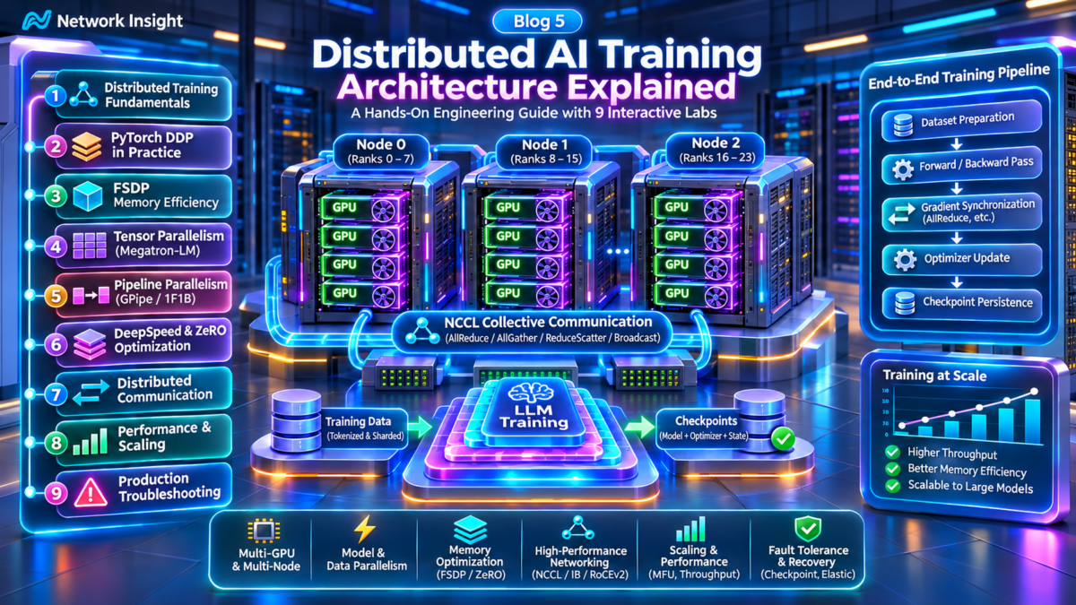
Distributed AI Training Architecture: From GPU Workers to Synchronized Model Updates
Distributed AI training coordinates computation across multiple GPUs and compute nodes to process large datasets, train increasingly complex models and reduce training time. The architecture combines model execution, distributed communication, accelerator memory, data pipelines and orchestration.
At the heart of distributed training is a repeated execution cycle: input data enters participating workers, model computation produces a loss, gradients are calculated and the training system coordinates the information required to update model parameters.
Distributed Training Overview
Multiple GPU workers execute coordinated training steps, exchange required information and update model state.
Distributed training improves capacity and potential throughput, but communication and synchronization overhead influence scaling efficiency.
The Distributed Training Execution Model
A distributed training job consists of participating processes, commonly identified by ranks. Each rank executes part of the training workload using the accelerator resources assigned to it. Processes communicate through configured process groups and collective communication operations.
From Forward Pass to Parameter Update
During the forward pass, the model processes input data and produces predictions. A loss function evaluates the output against the training objective. Backward propagation then computes gradients for trainable parameters.
In conventional synchronous data parallelism, workers coordinate gradient information before applying optimizer updates. Other strategies, including fully sharded and tensor-parallel execution, use different communication and state-partitioning patterns.
Important distinction: The diagram represents a synchronous data-parallel training pattern. It does not imply that every distributed training system uses one central gradient aggregation service or a centralized optimizer. In typical DDP training, collective communication and optimizer updates are performed by the participating processes.
Why Communication Architecture Matters
Distributed training performance depends on the relationship between useful computation and the time spent exchanging information. Network bandwidth, communication latency, collective algorithms and accelerator topology can all influence the duration of a training step.
As model size and GPU count increase, engineers must choose parallelism strategies that balance memory requirements, computation and communication overhead.
Architecture is illustrative. Actual rank placement, GPU counts, communication groups, model partitioning and checkpoint strategies depend on the distributed training framework and deployment.
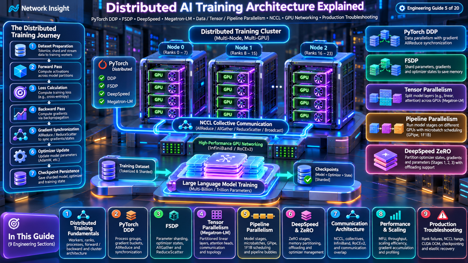
Explore Distributed AI Training Architecture
Navigate nine engineering layers of large-scale model training, from distributed workers and tensor sharding to NCCL communication, scaling analysis and production recovery. Select any architecture node to inspect the topic and open its corresponding section.
Distributed Training Fundamentals
Explore worker ranks, process groups and synchronized distributed training execution.
Distributed AI Training Architecture: From GPU Workers to Synchronized Model Updates
Distributed AI training coordinates computation across multiple GPUs and compute nodes to process large datasets, train increasingly complex models and reduce training time. The architecture combines model execution, distributed communication, accelerator memory, data pipelines and orchestration.
At the heart of distributed training is a repeated execution cycle: input data enters participating workers, model computation produces a loss, gradients are calculated and the training system coordinates the information required to update model parameters.
Distributed Training Overview
Multiple GPU workers execute coordinated training steps, exchange required information and update model state.
Distributed training improves capacity and potential throughput, but communication and synchronization overhead influence scaling efficiency.
The Distributed Training Execution Model
A distributed training job consists of participating processes, commonly identified by ranks. Each rank executes part of the training workload using the accelerator resources assigned to it. Processes communicate through configured process groups and collective communication operations.
From Forward Pass to Parameter Update
During the forward pass, the model processes input data and produces predictions. A loss function evaluates the output against the training objective. Backward propagation then computes gradients for trainable parameters.
In conventional synchronous data parallelism, workers coordinate gradient information before applying optimizer updates. Other strategies, including fully sharded and tensor-parallel execution, use different communication and state-partitioning patterns.
Important distinction: The diagram represents a synchronous data-parallel training pattern. It does not imply that every distributed training system uses one central gradient aggregation service or a centralized optimizer. In typical DDP training, collective communication and optimizer updates are performed by the participating processes.
Why Communication Architecture Matters
Distributed training performance depends on the relationship between useful computation and the time spent exchanging information. Network bandwidth, communication latency, collective algorithms and accelerator topology can all influence the duration of a training step.
As model size and GPU count increase, engineers must choose parallelism strategies that balance memory requirements, computation and communication overhead.
Architecture is illustrative. Actual rank placement, GPU counts, communication groups, model partitioning and checkpoint strategies depend on the distributed training framework and deployment.
Distributed Training Architecture Explorer
Explore how training processes execute across GPU nodes. Follow dataset sharding, forward computation, loss calculation, backward propagation, gradient synchronization and optimizer updates across distributed ranks.
Distributed training cluster architecture
Select a GPU worker to inspect its global rank, local rank, node assignment and training role.
Configure the cluster and begin a synchronized training step.
Each GPU runs one training process in this simplified data-parallel configuration. All processes participate in the same distributed process group.
PyTorch DDP Architecture: Gradient Buckets, Backward Hooks, NCCL AllReduce and Synchronized Optimizer Updates
PyTorch Distributed Data Parallel (DDP) is a distributed training mechanism that maintains model replicas across participating processes and synchronizes their gradients during backward propagation.
DDP integrates with PyTorch autograd, organizes gradients into communication buckets and uses collective operations to coordinate training across GPUs and compute nodes.
Replicated Model Architecture
Each participating process maintains a model replica and processes its own input batch.
DDP synchronizes gradients, while optimizer updates normally occur independently on each rank using the synchronized values.
Interactive AllReduce Gradient Calculation
Enter four scalar gradients to illustrate a sum-reduction followed by averaging across four equally weighted workers.
1. DDP Architecture and Model Replication
PyTorch DDP wraps a model so participating processes can execute training on separate inputs while coordinating gradients.
In a common GPU configuration, each process owns one GPU and maintains a complete model replica.
2. Process Group Initialization
Distributed processes initialize a communication group with rank and world-size information. The NCCL backend is commonly used for GPU collective communication.
Correct device selection, process membership and initialization configuration are essential for reliable execution.
3. Forward Computation
Each DDP worker executes a forward pass on its local input batch. The model produces outputs, and the loss function calculates the training objective.
DDP does not ordinarily exchange full activations between replicas during conventional data-parallel forward computation.
4. Autograd Hooks and Gradient Buckets
DDP integrates with autograd and tracks when parameter gradients become ready during backward computation.
Gradients are organized into buckets to support efficient communication. When a bucket is ready, its reduction can begin without waiting for the entire backward pass to finish.
Engineering distinction: Gradient bucketing enables communication to overlap with backward computation. The amount of overlap depends on gradient readiness, bucket composition, communication performance and the training workload.
5. NCCL AllReduce Gradient Synchronization
AllReduce combines gradient contributions across participating processes and makes the reduced result available to each participant.
In conventional DDP configurations, gradients are averaged across the participating workers, accounting for the framework's reduction behavior and loss scaling.
Collective algorithms may use ring, tree or other topology-aware strategies depending on the backend and deployment.
6. Optimizer Updates
After required gradient synchronization completes, each worker applies its optimizer step using its local optimizer and synchronized gradients.
With consistent initial model and optimizer states and equivalent updates, replicas remain synchronized.
7. DDP Performance Engineering
DDP performance depends on the balance between GPU computation and gradient communication.
Network bandwidth, collective latency, bucket configuration, model architecture and batch size can affect scaling efficiency.
8. Common DDP Failure Conditions
Distributed jobs may stall because of mismatched collective participation, worker failure, network problems, process initialization errors or uneven execution behavior.
Effective troubleshooting requires correlating rank-level logs, process health and communication telemetry.
| DDP component | Purpose | Engineering consideration |
|---|---|---|
| Model replica | Executes local model computation | Consistent parameters and device placement |
| Autograd | Computes parameter gradients | Backward execution and gradient readiness |
| Gradient bucket | Groups gradients for communication | Bucket sizing and overlap |
| AllReduce | Combines gradient contributions | Communication latency and throughput |
| NCCL backend | GPU collective communication | Network and accelerator topology |
| Optimizer | Updates model parameters | Consistent state and gradient scaling |
9. Engineering Takeaway
PyTorch DDP is a replicated-model training architecture that coordinates gradients rather than centrally updating all model parameters.
Understanding gradient buckets, autograd hooks, collective communication and optimizer execution provides the foundation for evaluating more memory-efficient approaches such as Fully Sharded Data Parallel and DeepSpeed ZeRO.
The numerical example assumes four equally weighted scalar gradients. Real DDP behavior also depends on loss reduction, gradient accumulation, synchronization configuration and process-group membership.
DDP Gradient Synchronization Visualizer
Investigate gradient bucket readiness, NCCL AllReduce and communication overlap across distributed training ranks. Compare the effects of bucket size, backward computation and effective collective bandwidth.
Gradient bucket and collective communication architecture
DDP groups parameter gradients into buckets. When all gradients belonging to a bucket are ready, its collective synchronization can be launched.
Start the backward pass to examine bucket synchronization.
Smaller buckets can enable earlier communication, but introduce more collective launches. Larger buckets reduce launch count but may delay readiness.
PyTorch FSDP Architecture: Parameter Sharding, AllGather, ReduceScatter and GPU Memory Optimization
Fully Sharded Data Parallel (FSDP) reduces the persistent GPU memory required for distributed model training by partitioning model parameters, gradients and optimizer states across participating workers.
Unlike conventional DDP, which maintains complete model replicas and optimizer state on each rank, fully sharded training distributes these states and temporarily gathers the parameters needed for computation.
Persistent Parameter Shards
Each participating rank stores a partition of the model parameters rather than a complete persistent replica.
Sharding reduces persistent memory requirements, but communication and temporary parameter materialization still consume resources.
DDP vs FSDP Model-State Memory Calculator
Estimate persistent parameter, gradient and optimizer-state memory per GPU under a simplified fully sharded configuration.
1. Why Fully Sharded Data Parallel Exists
Large neural networks require substantial accelerator memory for parameters, gradients, optimizer states and intermediate activations.
Conventional DDP replicates the model and optimizer state across participating workers, which can make memory capacity a limiting factor.
2. FSDP Model-State Partitioning
FSDP distributes persistent model parameters, gradients and optimizer state across a group of participating processes.
Each rank maintains its assigned shards and participates in collective communication to obtain the parameters needed for computation.
3. Parameter AllGather
Before a sharded module executes, participating ranks may perform an AllGather operation to materialize the required full parameter set.
This communication exchanges parameter shards among workers so computation can proceed using the necessary model weights.
4. Forward Computation and Resharding
Once the required parameters are available, the module executes its forward computation.
Depending on the FSDP configuration and implementation, full parameters can be released or resharded after forward execution to reduce memory pressure.
Engineering distinction: FSDP reduces persistent model-state memory, not all GPU memory. Activations, temporary full parameters, communication buffers and other runtime allocations still contribute to peak memory consumption.
5. Backward Propagation and Gradient Communication
Backward computation requires the relevant model parameters and produces parameter gradients.
Fully sharded execution commonly uses ReduceScatter to combine gradient contributions and distribute the resulting gradient shards among participating workers.
6. Sharded Optimizer State
Each worker maintains optimizer state for its assigned parameter shards rather than storing a complete optimizer state for every model parameter.
For optimizers with substantial auxiliary state, such as Adam, optimizer-state sharding can provide significant persistent memory savings.
7. FSDP Memory Engineering
A simplified persistent model-state estimate divides the total sharded model state by the number of participating ranks.
Real GPU memory consumption also depends on parameter precision, optimizer implementation, activation checkpointing, module wrapping, prefetching and temporary parameter materialization.
8. FSDP Communication Tradeoffs
FSDP reduces memory replication at the cost of additional communication, especially parameter AllGather operations.
Performance depends on communication overlap, network bandwidth, module boundaries, sharding configuration and the balance between computation and data movement.
| Characteristic | Conventional DDP | Fully Sharded Data Parallel |
|---|---|---|
| Persistent parameters | Replicated per worker | Partitioned across workers |
| Persistent gradients | Replicated after synchronization | Partitioned in fully sharded execution |
| Optimizer state | Replicated per worker | Partitioned across workers |
| Primary communication | Gradient AllReduce | Parameter AllGather and gradient ReduceScatter |
| Memory efficiency | Limited by replicated model state | Reduced persistent model-state memory |
| Communication tradeoff | Gradient synchronization | Additional parameter gathering |
9. Engineering Takeaway
FSDP enables larger models to train across distributed GPUs by partitioning persistent model state while dynamically gathering parameters needed for execution.
Its value comes from reducing memory replication, but successful deployment requires careful consideration of collective communication, peak memory and model execution patterns.
The calculator uses decimal GB and an idealized equal-sharding model. It is not a GPU capacity planner and excludes activations, temporary full parameters, communication buffers, fragmentation and framework-specific overhead.
FSDP Memory and Sharding Explorer
Compare replicated model state with fully sharded training. Investigate how parameters, gradients and optimizer states are distributed across ranks, and trace AllGather, forward execution, resharding and ReduceScatter operations.
Distributed model-state architecture
Fully sharded training distributes persistent parameter, gradient and optimizer state across ranks. Parameters are temporarily gathered when required for computation.
Configure the model and begin the FSDP lifecycle.
FSDP reduces persistent state memory but introduces parameter-gather and gradient-reduction communication. Activation memory is not included in this estimate.
Tensor Parallelism Architecture: Partitioned Linear Layers, Attention Heads, Megatron-LM and GPU Communication
Tensor parallelism distributes the computation of individual neural-network layers across multiple GPUs. Instead of assigning complete model layers or complete replicas to separate workers, tensor parallelism partitions weight matrices and intermediate computation.
This approach is important when individual layers are too large for one accelerator or when engineers want to distribute large matrix operations across a tightly connected GPU group.
Partitioned Model Tensors
Large weight matrices are divided across GPUs, with each GPU responsible for a portion of the layer computation.
Tensor parallelism distributes individual layer computation, unlike data parallelism, which distributes input batches across model replicas.
Tensor Parallel Sharding Calculator
Explore how a simple column-parallel linear layer partitions output features and attention heads across a tensor-parallel group.
1. What Is Tensor Parallelism?
Tensor parallelism divides the computation of individual neural-network layers across multiple GPUs.
Each worker holds part of a layer's weights and performs the corresponding matrix operations. Communication combines or redistributes intermediate results when required.
2. Tensor Parallelism vs Data Parallelism
Data parallelism assigns different training examples to replicated model computation. Tensor parallelism partitions the operations within a model layer.
Both approaches can be combined in large-scale training systems to balance memory capacity, computation and communication.
3. Column-Parallel Linear Layers
For a linear transformation, a column-parallel layout partitions the output-feature dimension of the weight matrix.
Each GPU computes a subset of output features. The resulting output tensors may remain partitioned or be gathered, depending on the next operation.
4. Row-Parallel Linear Layers
A row-parallel layout partitions the input-feature dimension of a linear layer. Each worker computes a partial contribution to the output.
When the desired output is replicated, the partial contributions can be combined using a reduction operation such as AllReduce.
Engineering distinction: Column-parallel layers partition output features, while row-parallel layers partition input features. Their communication requirements depend on whether input and output tensors are replicated or sharded.
5. Attention-Head Partitioning
Multi-head attention provides a natural opportunity for tensor parallelism because different attention heads can be computed independently before their outputs are combined.
In a compatible architecture, attention heads are assigned across participating GPUs. Grouped-query attention and other transformer variants can introduce additional placement constraints.
6. Megatron-LM Transformer Execution
Megatron-style tensor parallelism commonly combines column-parallel and row-parallel operations within transformer attention and feed-forward blocks.
This arrangement allows intermediate tensors to remain partitioned between selected operations, reducing unnecessary communication.
7. Collective Communication Architecture
Tensor parallelism uses collective communication to exchange or combine intermediate tensors.
Depending on the implementation, operations may include AllReduce, AllGather and ReduceScatter. Communication occurs during both forward and backward computation.
8. GPU Topology and Performance
Tensor-parallel workers frequently exchange intermediate data, making communication bandwidth and latency important.
High-bandwidth intra-node interconnects such as NVLink and NVSwitch can be advantageous for tightly coupled tensor-parallel groups. Larger deployments may also use inter-node communication.
| Architecture | Partitioning strategy | Communication requirement |
|---|---|---|
| Data parallelism | Input batches across replicas | Gradient synchronization |
| Column parallel | Output-feature dimension | Optional output gathering and backward communication |
| Row parallel | Input-feature dimension | Reduction of partial outputs where required |
| Attention heads | Head computation across GPUs | Depends on projection and output layout |
| Megatron-style TP | Transformer layer tensor partitions | Topology-aware collective operations |
| Hybrid parallelism | Tensor, data and pipeline dimensions | Multiple communication groups |
9. Engineering Takeaway
Tensor parallelism enables large neural-network layers to execute across multiple GPUs by distributing weight matrices and intermediate computation.
Its effectiveness depends on selecting compatible tensor layouts, minimizing unnecessary collective communication and placing tightly coupled GPU workers on suitable interconnects.
The calculator assumes equal partitioning of a simplified column-parallel projection and evenly divisible attention heads. Real models may have separate query/key/value head counts, padding constraints, fused projections and implementation-specific tensor layouts.
Tensor Parallel Execution Explorer
Explore how large matrix operations and attention heads are partitioned across GPUs. Trace local tensor computation, collective communication and distributed output construction using Megatron-LM-style tensor parallelism.
Distributed tensor computation architecture
Tensor parallelism divides individual model operations across multiple GPUs. Each rank computes a local partition and participates in communication when the next operation requires a combined result.
Choose an operation and execute its distributed stages.
Column-parallel and row-parallel layers have different forward communication requirements. Attention-head partitioning distributes independent heads when their dimensions are compatible.
Pipeline Parallelism Architecture: Model Stages, Microbatches, GPipe, 1F1B Scheduling and Pipeline Bubbles
Pipeline parallelism divides a neural network into sequential stages placed on different GPUs or groups of GPUs. Instead of requiring one accelerator to execute the complete model, each pipeline stage processes its assigned layers and transfers intermediate activations to the next stage.
By splitting training batches into microbatches, multiple pipeline stages can execute concurrently. Scheduling determines when forward and backward operations run, how much activation memory is retained and how much time GPUs spend idle.
GPipe Execution
All microbatches complete their forward passes before backward execution begins.
GPipe is straightforward to schedule, while 1F1B can reduce the number of outstanding activations.
Simulation assumes equal-duration forward and backward operations, zero transfer latency, one operation per stage per time slot and no interleaving of virtual pipeline stages. These are illustrative schedule metrics, not measured training performance.
1. Pipeline Parallel Architecture
Pipeline parallelism partitions a model by layer or block boundaries. A stage executes its assigned model operations and sends activations to the next stage during forward propagation.
During backward propagation, gradient information flows in the opposite direction. Each stage calculates the gradients associated with its own parameters.
2. Microbatch Execution
A training batch is divided into smaller microbatches. This permits multiple pipeline stages to work simultaneously on different microbatches.
Increasing the number of microbatches can improve stage utilization, although smaller microbatches may change GPU kernel efficiency and memory behavior.
3. GPipe Fill-Drain Scheduling
GPipe-style scheduling first fills the pipeline with forward operations. Once forward computation has completed for the microbatches, backward operations drain the pipeline.
This schedule is conceptually simple but can require substantial activation storage because several microbatches may be awaiting backward execution.
4. 1F1B Pipeline Scheduling
One-forward-one-backward scheduling interleaves forward and backward operations after a warmup phase. Each stage alternates between processing forward and backward work where dependencies permit.
Compared with fill-drain execution, 1F1B can reduce the maximum number of outstanding activations. Its precise execution order depends on the pipeline implementation.
Engineering distinction: 1F1B does not automatically eliminate pipeline bubbles. Both GPipe and non-interleaved 1F1B have warmup and drain overhead. Under common idealized equal-stage assumptions, they can have similar total makespans even though their activation-memory behavior differs.
5. Pipeline Bubbles and Utilization
A pipeline bubble occurs when a stage has no useful work because the necessary inputs or gradients are not yet available.
For a simple pipeline with P stages and M microbatches, an often-used idealized bubble fraction is approximately (P − 1) / (M + P − 1), under the relevant equal-duration and non-interleaved scheduling assumptions.
Increasing microbatch count can reduce the relative bubble fraction, but practical throughput also depends on kernel efficiency, communication, memory and load balance.
6. Activation Memory and Checkpointing
Each pipeline stage may retain forward activations until its corresponding backward operation completes. The number of outstanding microbatches therefore influences activation memory requirements.
Activation checkpointing can trade additional recomputation for lower memory usage, making larger models or more microbatches feasible.
7. Pipeline Communication
Adjacent stages exchange activations during forward computation and activation gradients during backward computation. These transfers typically use point-to-point communication.
Pipeline placement should consider interconnect bandwidth, message sizes, stage boundaries and the cost of moving tensors between nodes.
8. Pipeline Performance Engineering
Pipeline efficiency depends on stage balance, microbatch count, communication overhead, activation memory and the scheduling strategy.
Hybrid distributed training systems often combine pipeline parallelism with tensor parallelism and data parallelism, each using separate communication groups.
| Characteristic | GPipe | Non-interleaved 1F1B |
|---|---|---|
| Forward/backward order | Forward phase, then backward phase | Warmup, interleaved steady state, drain |
| Activation residency | Potentially more outstanding microbatches | Often fewer outstanding microbatches |
| Pipeline bubbles | Fill and drain overhead | Warmup and drain overhead |
| Communication | Adjacent-stage activation transfers | Adjacent-stage activation transfers |
| Complexity | Relatively straightforward | More scheduling dependencies |
| Primary optimization | Microbatch count and balanced stages | Activation residency and balanced stages |
9. Engineering Takeaway
Pipeline parallelism enables large neural networks to span multiple accelerators by partitioning model layers into stages and overlapping the execution of microbatches.
The central design challenge is balancing pipeline utilization against activation memory, communication overhead and scheduling complexity.
This educational timeline models conventional fill-drain and a dependency-aware non-interleaved 1F1B schedule. Actual implementations may use interleaved stages, different operation durations, communication overlap and additional synchronization.
Pipeline Schedule Timeline
Visualize how model layers are divided across GPUs and how microbatches move through forward and backward computation. Compare GPipe and 1F1B execution schedules, investigate pipeline bubbles and identify the impact of stage imbalance.
Pipeline-parallel GPU architecture
Forward and backward execution timeline
GPipe schedules all forward microbatches before backward computation. 1F1B interleaves forward and backward work after warm-up.
Build a schedule to investigate forward/backward dependencies and GPU idle periods.
Increasing the number of microbatches can amortize pipeline fill and drain overhead, but may affect activation storage, kernel efficiency and communication.
DeepSpeed ZeRO Architecture: Optimizer-State Sharding, Gradient Partitioning, Parameter Sharding and CPU/NVMe Offloading
DeepSpeed ZeRO, or Zero Redundancy Optimizer, reduces the memory duplication traditionally associated with distributed data-parallel training. It progressively partitions optimizer states, gradients and model parameters across participating data-parallel workers.
ZeRO Stages 1, 2 and 3 provide different memory and communication tradeoffs. DeepSpeed also supports offloading selected model states to CPU memory and, in supported configurations, NVMe storage.
Conventional DDP Baseline
Every data-parallel worker holds a complete persistent copy of parameters, gradients and optimizer state.
ZeRO reduces redundancy by progressively sharding persistent model state, but increases coordination requirements.
ZeRO Persistent Model-State Memory Calculator
Compare the estimated per-GPU persistent model-state memory for DDP and each ZeRO stage, using a simplified mixed-precision Adam-style accounting model.
1. The Model-State Redundancy Problem
Conventional data-parallel training replicates model parameters, gradients and optimizer state across participating workers. For large models, optimizer states and master weights can occupy substantially more memory than the low-precision model weights alone.
ZeRO addresses this redundancy by distributing persistent state across the data-parallel group while preserving the mathematical requirements of distributed optimization.
2. ZeRO Stage 1: Optimizer-State Partitioning
ZeRO-1 partitions optimizer state across data-parallel workers. Each rank owns optimizer state for a subset of parameters, while model parameters and gradients remain replicated in the conventional stage-1 arrangement.
After the appropriate updates, parameter values are coordinated so workers continue training with consistent model state.
3. ZeRO Stage 2: Gradient Partitioning
ZeRO-2 extends optimizer-state partitioning by distributing gradient storage across participating ranks. Each rank retains the reduced gradients associated with its assigned parameter partition.
Collective communication, including reduction and partitioning mechanisms, supports the sharded optimizer update. Model parameters remain replicated.
4. ZeRO Stage 3: Parameter Partitioning
ZeRO-3 additionally partitions model parameters, eliminating the requirement for every rank to persistently store all model weights.
Workers gather required parameter partitions during execution and release or repartition temporary materializations according to the implementation and configuration.
Engineering distinction: ZeRO-3 and fully sharded data-parallel approaches share the fundamental idea of sharding parameters, gradients and optimizer states. They are not necessarily identical implementations: execution scheduling, parameter management, communication overlap, offloading and checkpoint handling may differ.
5. CPU Offloading
DeepSpeed supports configurations that move selected optimizer state and/or parameter state into CPU memory. This can reduce GPU memory pressure and enable larger models on limited accelerator capacity.
However, CPU offloading introduces transfers across the CPU–GPU interconnect and may shift computation or state management to the host. Throughput depends on transfer volume, CPU performance, pinned memory, overlap and available system RAM.
6. NVMe Offloading
Supported DeepSpeed offload configurations can use NVMe storage as an additional capacity tier for selected model state.
NVMe offers more capacity than GPU memory but has substantially different latency and bandwidth characteristics. Prefetching, buffering, transfer scheduling and storage performance become critical.
7. Memory and Communication Tradeoffs
As ZeRO progresses from Stage 1 to Stage 3, persistent model-state redundancy decreases. In exchange, the runtime performs additional distributed coordination and may gather or redistribute model parameters.
Offloading adds another tradeoff: GPU memory savings in exchange for data transfers, host resources and potentially storage I/O. The fastest configuration is not necessarily the configuration with the smallest GPU memory footprint.
8. Production Troubleshooting
ZeRO training failures may involve collective mismatches, CPU RAM exhaustion, GPU out-of-memory conditions during parameter materialization, insufficient NVMe capacity, slow offload transfers or checkpoint reconstruction problems.
Engineers should monitor GPU allocated and peak memory, CPU memory pressure, interconnect throughput, collective duration, NVMe I/O and rank-level failures.
| Architecture | Parameters | Gradients | Optimizer state | Primary tradeoff |
|---|---|---|---|---|
| DDP baseline | Replicated | Replicated | Replicated | High model-state memory use |
| ZeRO Stage 1 | Replicated | Replicated | Sharded | Optimizer partition coordination |
| ZeRO Stage 2 | Replicated | Sharded | Sharded | Gradient partition communication |
| ZeRO Stage 3 | Sharded | Sharded | Sharded | Parameter gathering and coordination |
| CPU offload | Configuration-dependent | Configuration-dependent | May reside on CPU | Host memory and transfer overhead |
| NVMe offload | Configuration-dependent | Configuration-dependent | May use NVMe | Storage I/O and transfer scheduling |
9. Engineering Takeaway
DeepSpeed ZeRO enables larger-scale model training by progressively eliminating redundant persistent model-state copies across data-parallel workers.
The engineering decision is not simply which stage saves the most memory. It is which combination of sharding, communication, host resources and offloading delivers a viable balance of model capacity, throughput and operational reliability.
The memory calculator assumes 2-byte model parameters, 2-byte gradients and 12 bytes of optimizer/master state per parameter, with equal partitioning and no offload. Real precision modes, optimizers, memory layouts, parameter persistence thresholds and framework implementations can produce different results. Figures use decimal GB.
ZeRO Memory Optimization Explorer
Investigate how DeepSpeed ZeRO partitions optimizer states, gradients and parameters across training ranks. Compare GPU memory consumption, examine offloading strategies and trace the communication operations introduced by ZeRO optimization.
Distributed GPU model-state memory architecture
ZeRO progressively eliminates redundant model-state copies across data-parallel ranks.
Configure the ZeRO stage and begin a training step.
Higher ZeRO stages reduce persistent GPU memory at the cost of additional communication and potentially higher execution overhead.
Distributed Training Communication: NCCL, AllReduce, AllGather, ReduceScatter, NVLink, InfiniBand and RoCEv2
Distributed AI training depends on a communication architecture that moves gradients, model parameters, activations and other tensors between participating GPU workers. Communication performance influences training throughput, scaling efficiency and the ability to execute large models across multiple compute nodes.
NCCL provides GPU-oriented collective communication, while high-bandwidth intra-node interconnects and RDMA-capable network fabrics support data movement within and between GPU servers.
Distributed GPU Fabric Architecture
GPU workers communicate through intra-node interconnects and inter-node network adapters connected to a cluster fabric.
Distributed training performance depends on the complete communication path, not simply the nominal link speed.
Collective Communication Bandwidth Calculator
Estimate the bandwidth-limited communication time for a ring AllReduce using an idealized per-rank transfer-volume model.
1. Distributed Training Communication Fundamentals
Distributed training systems exchange model parameters, gradients, activations and optimizer-related information between participating processes.
The communication pattern depends on whether the workload uses data parallelism, tensor parallelism, pipeline parallelism or a combination of strategies.
2. NCCL Collective Communication
NVIDIA Collective Communications Library (NCCL) provides collective operations optimized for supported GPU environments.
NCCL selects communication strategies according to the operation, participating devices, topology and available transports. Collective communication may use multiple channels and different algorithms.
3. AllReduce Architecture
AllReduce combines contributions from participating ranks using a reduction operation and makes the reduced result available to each rank.
Gradient synchronization in conventional DDP is a common example. Implementations may use ring, tree or other algorithms depending on topology and workload characteristics.
4. AllGather and ReduceScatter
AllGather collects distributed tensor partitions and makes the gathered result available to participating ranks.
ReduceScatter reduces distributed contributions and distributes partitions of the result. These operations are important for fully sharded training and some tensor-parallel execution patterns.
Engineering distinction: NCCL defines collective communication behavior, but the physical transport can differ. Intra-node GPU communication may use NVLink or PCIe paths, while inter-node traffic may traverse InfiniBand or RoCE-capable Ethernet infrastructure.
5. Intra-Node GPU Communication
GPU servers may use NVLink, NVSwitch and PCIe to connect accelerators and other components. These technologies have different bandwidth, latency and topology characteristics.
Collective performance depends on the available paths between participating GPUs, the system architecture and the communication algorithm.
6. InfiniBand and RoCEv2
InfiniBand provides a high-performance network fabric with RDMA capabilities commonly used in large AI clusters.
RoCEv2 transports RDMA traffic over Ethernet/IP networks. Its operational design requires attention to congestion management, queueing, packet loss, ECN and priority flow control where deployed.
7. RDMA and GPU Data Movement
RDMA allows supported systems to transfer data between memory regions with reduced CPU involvement in the data path.
GPUDirect RDMA can enable supported network adapters to access GPU memory directly, subject to platform, topology, driver and software requirements.
8. Communication Overlap
Distributed training frameworks can overlap collective communication with GPU computation to reduce exposed communication time.
For example, DDP may begin reducing ready gradient buckets while backward computation continues. The effectiveness of overlap depends on the critical path, resource contention and communication scheduling.
| Technology / operation | Primary role | Engineering consideration |
|---|---|---|
| NCCL | GPU collective communication | Algorithm, topology and transport selection |
| NVLink / NVSwitch | Intra-node GPU connectivity | GPU-to-GPU bandwidth and topology |
| InfiniBand | RDMA-capable cluster network | Fabric design, routing and congestion |
| RoCEv2 | RDMA over Ethernet/IP | ECN, queueing, loss and PFC strategy |
| AllReduce | Reduce and distribute result | Collective latency and transfer volume |
| AllGather | Gather tensor partitions | Parameter materialization and memory |
| ReduceScatter | Reduce and partition result | Sharded gradient synchronization |
9. Engineering Takeaway
Distributed training communication performance depends on collective algorithms, GPU interconnects, network transport, topology and the ability to overlap data movement with useful computation.
For network engineers, understanding NCCL behavior alongside InfiniBand and RoCEv2 fabric design is essential for diagnosing slow training jobs and designing scalable AI infrastructure.
The calculator uses decimal MB and a simplified ring AllReduce transfer volume of 2 × (N − 1) / N × tensor size per rank. The resulting time is a bandwidth-only estimate, not a prediction of real NCCL collective latency.
Distributed Communication Timeline Analyzer
Investigate NCCL collective communication across GPU fabrics. Compare AllReduce, AllGather, ReduceScatter and Broadcast operations, model communication latency and bandwidth, and explore how congestion and computation overlap influence training performance.
GPU collective communication topology
AllReduce aggregates distributed values and makes the reduced result available to participating ranks.
Run an analysis to inspect the collective communication path.
Bandwidth dominates large-message collectives, while startup latency and synchronization overhead become important for smaller messages.
Distributed Training Performance: GPU Scaling Efficiency, Model FLOPs Utilization, Throughput and Bottleneck Investigation
Scaling distributed AI training requires more than adding accelerators. Performance depends on how effectively the system converts GPU compute capacity into useful model operations while minimizing communication stalls, input-pipeline delays, synchronization overhead and memory-related inefficiencies.
Engineering teams evaluate training throughput, scaling efficiency, Model FLOPs Utilization (MFU), communication overlap and GPU profiling data to identify where training time is being lost.
Training Pipeline Overview
Training throughput depends on the complete execution path from data loading to GPU computation, communication and optimizer updates.
High accelerator utilization does not necessarily imply high Model FLOPs Utilization or efficient distributed scaling.
Scaling Efficiency and MFU Calculator
Estimate strong-scaling efficiency and Model FLOPs Utilization using measured training throughput and an explicitly supplied model-FLOPs estimate.
1. Distributed Training Performance Fundamentals
Distributed training performance is determined by the rate at which a cluster processes useful training work, commonly measured as samples or tokens per second.
Increasing GPU count expands available compute capacity, but communication, synchronization and input-pipeline overhead can prevent proportional throughput growth.
2. Strong Scaling and Weak Scaling
Strong scaling measures performance improvement when a fixed workload is distributed across more processing resources.
Weak scaling examines performance as the workload grows alongside the number of processing resources. The two approaches answer different capacity-planning questions.
3. Scaling Efficiency
Strong-scaling efficiency compares observed speedup with ideal linear speedup. If eight GPUs deliver 6.2 times the throughput of a single GPU for a comparable workload, efficiency is approximately 77.5%.
Scaling efficiency may decline as communication overhead, synchronization and workload imbalance increase.
4. Model FLOPs Utilization
Model FLOPs Utilization (MFU) compares the estimated floating-point operations required for useful model computation per second against the theoretical peak compute capability of the participating GPUs.
MFU is different from GPU activity metrics. A GPU can report high activity while spending substantial time on operations that do not translate into high useful model FLOPs throughput.
Engineering distinction: MFU calculations require a defensible model-FLOPs estimate and the correct peak compute specification for the relevant precision and hardware configuration. A simplified FLOPs-per-token estimate can be useful, but it is not a substitute for a validated model-specific FLOPs accounting methodology.
5. Communication Overhead
Distributed training may spend significant time exchanging gradients, parameters and activations. Communication overhead depends on collective algorithms, network bandwidth, latency and topology.
Communication overlap can reduce exposed waiting time, but network contention and collective scheduling can still limit throughput.
6. GPU Idle Time and Input Bottlenecks
GPUs may remain idle while waiting for data loading, preprocessing, storage reads, synchronization or slower workers.
Performance engineers should examine data-loader worker utilization, CPU saturation, storage throughput and step-level timing rather than assuming the GPU is always the bottleneck.
7. Gradient Accumulation
Gradient accumulation combines gradients across multiple microbatches before applying an optimizer update. It can increase effective batch size without requiring the entire batch to fit in GPU memory at once.
Accumulation changes optimizer-step frequency relative to microbatch execution. Communication behavior depends on the training framework and whether synchronization is deferred during intermediate microbatches.
8. Performance Profiling
Useful profiling data includes GPU kernel timelines, collective durations, CPU execution, memory allocation, data-loading latency and synchronization events.
Engineers should correlate GPU traces with network telemetry and training-step metrics to identify the actual critical path.
| Metric | What it measures | Engineering interpretation |
|---|---|---|
| Training throughput | Samples or tokens processed per second | End-to-end useful training rate |
| Strong-scaling efficiency | Observed speedup / GPU count | How close scaling is to ideal linear behavior |
| MFU | Useful model FLOPs / theoretical peak FLOPs | Model compute efficiency |
| Collective duration | Time spent in distributed communication | Communication bottlenecks and synchronization |
| GPU idle time | Time without useful GPU execution | Potential data, synchronization or scheduling stalls |
| Gradient accumulation | Microbatches per optimizer update | Effective batch-size and synchronization tradeoffs |
9. Engineering Takeaway
Distributed training performance engineering requires a complete understanding of GPU computation, communication, memory and data-pipeline behavior.
The most effective optimization is usually the one that reduces time on the measured critical path, rather than simply increasing GPU count or nominal network bandwidth.
The calculator assumes comparable single-GPU and cluster workloads, and treats the supplied model FLOPs/token as useful model computation. Gradient accumulation is included as a configuration input for discussion but does not automatically alter the supplied measured throughput or MFU calculation.
Distributed Training Scaling Investigator
Investigate strong and weak scaling across GPU clusters. Model training throughput, compute efficiency, communication overhead, memory pressure and gradient accumulation, then diagnose the limiting factor in a distributed training workload.
Distributed GPU scaling architecture
Strong scaling keeps total workload fixed while increasing GPU count. Weak scaling increases workload with the number of GPUs.
Configure the distributed training cluster and run the experiment.
Increasing GPU count does not guarantee proportional throughput because communication, synchronization and workload granularity influence scaling efficiency.
Distributed AI Training Troubleshooting: NCCL Hangs, Rank Failures, CUDA OOM, Network Congestion and Checkpoint Recovery
Production distributed training introduces failure modes that do not occur in single-GPU execution. A failure in one worker can disrupt collective communication, block synchronization or cause an entire training job to terminate.
Reliable operations require rank-level observability, GPU and network telemetry, checkpoint integrity, failure classification and a recovery strategy appropriate to the distributed training framework.
Healthy Distributed Training
All ranks are participating in distributed training and collective operations are completing successfully.
A healthy baseline is essential for comparing performance and diagnosing future incidents.
1. Distributed Training Failure Architecture
Distributed training jobs contain multiple processes participating in coordinated computation and communication. A failure in one rank can prevent other ranks from completing collective operations.
Engineers must distinguish the first failing process from secondary symptoms appearing elsewhere in the cluster.
2. NCCL Collective Hangs
A collective may appear to hang when ranks do not enter compatible collective operations, when a rank stops progressing or when communication fails.
Possible causes include mismatched collective order, process failure, transport problems and resource exhaustion. A timeout message identifies a stalled operation but does not necessarily identify the original fault.
3. Rank and Process Failures
A distributed worker may terminate because of a software exception, GPU fault, operating-system resource limit, scheduler intervention or node failure.
Other ranks can subsequently fail or time out while waiting for synchronization. Incident analysis should correlate process exit codes, timestamps, node events and collective failures.
4. CUDA Out-of-Memory Errors
CUDA OOM occurs when a GPU cannot satisfy a memory allocation. Training memory consumption includes parameters, gradients, optimizer states, activations and temporary buffers.
Potential mitigations include reducing microbatch size, using activation checkpointing, changing precision where appropriate or introducing model-state sharding.
Engineering distinction: A collective timeout does not prove the network is faulty. One rank may have failed earlier due to CUDA OOM or another exception, leaving surviving ranks blocked in a collective. Always identify the earliest relevant failure across all ranks.
5. Network Congestion and Transport Failures
Inter-node communication can be affected by congestion, packet loss, adapter problems, topology imbalance or incorrect transport configuration.
For RoCEv2 deployments, engineers should correlate collective timing with ECN, PFC, interface counters, queue occupancy and packet-drop telemetry. InfiniBand environments require appropriate fabric and port-level diagnostics.
6. Checkpointing and Recovery
Distributed training checkpoints preserve sufficient state to resume training, potentially including model parameters, optimizer state, learning-rate scheduler state, random-number-generator state and progress metadata.
Checkpoint formats and recovery procedures depend on the framework, parallelism strategy and storage architecture. Sharded checkpoints require compatible reconstruction or redistribution when loading.
7. Elastic Training
Elastic training frameworks can support recovery from worker changes or failures under defined conditions. However, elasticity is not automatic for every distributed training configuration.
Recovery may require restarting workers, rebuilding process groups, restoring checkpoints and adjusting data sampling or optimizer state consistently.
8. Production Observability
Useful telemetry includes per-rank process state, GPU memory, kernel failures, collective operation timing, network adapter counters, node health, storage latency and checkpoint completion.
Correlating timestamps across these systems is essential for reconstructing the sequence of events during an incident.
| Failure | Typical symptom | First diagnostic priority | Potential recovery |
|---|---|---|---|
| NCCL hang | Collective timeout or stalled progress | Find earliest rank failure and collective mismatch | Correct root cause and restart affected job |
| Rank failure | Process exit or missing worker | Exit code, node events and application logs | Restart or supported elastic recovery |
| CUDA OOM | GPU allocation failure | Peak memory and allocation history | Reduce memory demand and restore checkpoint |
| Network congestion | Slow collectives or transport errors | Fabric counters and rank timing correlation | Resolve congestion or transport configuration |
| Checkpoint failure | Incomplete or unreadable saved state | Storage errors, metadata and checkpoint integrity | Restore last verified checkpoint |
| Node failure | Multiple ranks lost simultaneously | Scheduler and host-level events | Reschedule and resume from durable state |
9. Engineering Takeaway
Production distributed training reliability depends on the ability to correlate GPU, process, network and storage telemetry across all participating ranks.
The most important troubleshooting principle is to identify the first causal failure, rather than treating the final collective timeout or job termination as the root cause.
The console uses synthetic events and illustrative diagnostic commands. It does not execute commands, inspect a live cluster or perform recovery actions. Actual troubleshooting procedures depend on framework versions, deployment environment and security policies.
Distributed Training Incident Investigation Lab
Investigate production failures in distributed GPU training. Collect rank-level evidence, inspect NCCL communication, GPU memory, checkpoint state and orchestration events, identify the root cause and verify recovery.
Distributed training failure topology
Diagnostic investigation tools
Inject an incident to begin investigating a production distributed training failure.
All eight training ranks are healthy. No active incident.
Start by identifying which ranks are affected. Then correlate NCCL logs, GPU memory, network telemetry, checkpoint integrity and orchestration events.

- AI Inference Serving Architecture Explained - November 17, 2026
- Distributed AI Training Architecture Explained - November 17, 2026
- AI GPU Cluster Architecture Explained - November 17, 2026