
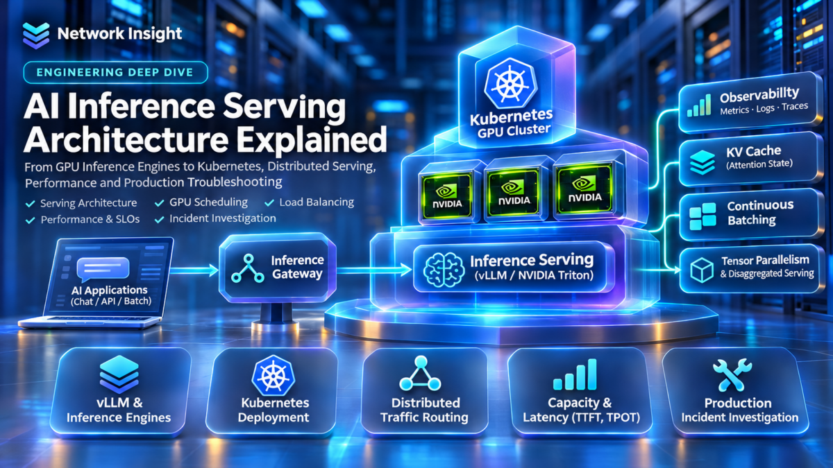
Inside a Production AI Inference Serving Platform
Every inference request travels through a coordinated system of API gateways, request schedulers, GPU model executors, memory managers and response-streaming services. Production performance depends on how efficiently these components transform incoming prompts into generated tokens.
This architecture explorer follows an illustrative request from the client to GPU execution and back, showing how vLLM, NVIDIA Triton, Kubernetes and GPU memory management fit into the serving stack.
Client Request
Applications submit prompts or inference payloads through an API endpoint. The request may include model selection, generation parameters and streaming preferences.
Conceptual architecture: specific request paths, batching mechanisms and model execution responsibilities vary by deployment and serving framework.
What Is AI Inference Serving?
AI inference serving is the infrastructure and software responsible for executing trained models in response to application requests. For autoregressive language models, this commonly involves processing the input prompt and generating output tokens iteratively.
Production serving systems coordinate request admission, model execution, GPU memory allocation, concurrency and response delivery to meet latency and throughput requirements.
Why Serving Architecture Matters
Inference workloads are highly variable. Requests can differ in prompt length, output length, model size and arrival time, creating scheduling and memory-management challenges.
Serving engines such as vLLM and model-serving platforms such as NVIDIA Triton provide mechanisms for managing execution and exposing models through service interfaces, while Kubernetes can orchestrate deployment and infrastructure resources.
Engineering perspective: Training systems optimize the rate of learning from data, whereas inference serving systems must balance response latency, throughput, concurrency, memory capacity and service reliability under changing request demand.
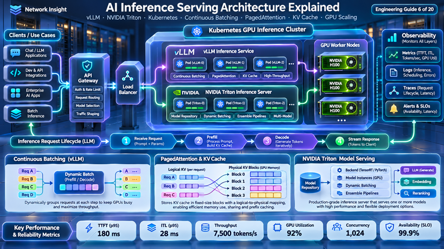
Explore the AI Inference Serving Architecture
Navigate nine engineering layers, from inference request handling and GPU memory to distributed serving, capacity planning and production troubleshooting.
Follow the inference request from client entry through scheduling, GPU execution and streamed token delivery.
Production AI Inference Architecture: Control Plane, Data Plane, Model Replicas and GPU Execution
Production AI inference platforms separate infrastructure orchestration from request execution. The control plane manages deployment configuration, model availability, scaling and lifecycle operations, while the data plane receives requests, schedules model execution and returns generated responses.
Understanding this separation is essential when designing scalable inference services using Kubernetes, vLLM, NVIDIA Triton or other model-serving technologies.
End-to-End Inference Request Flow
Inference requests enter through an application-facing endpoint, pass through routing and scheduling, execute on model-serving workers and return responses to clients.
The inference data plane processes live requests, while the control plane manages the resources and lifecycle of the serving infrastructure.
1. What Is an AI Inference Serving Platform?
An inference serving platform exposes trained models to applications through APIs or other service interfaces. It manages the execution environment, request processing and response delivery required to make models available to users and software systems.
For large language models, serving involves prompt processing, autoregressive token generation, attention-state management and potentially incremental response streaming.
2. Control Plane vs Data Plane
The control plane manages the deployment and operational lifecycle of model-serving infrastructure. Responsibilities can include replica management, configuration, scheduling onto infrastructure nodes and autoscaling.
The data plane handles live inference traffic, including request routing, batching, model execution and response delivery. The exact boundary varies by platform.
3. Inference Request Lifecycle
A typical inference request enters through an API gateway or serving endpoint, where authentication, quotas and routing policies may be applied.
The serving engine admits and schedules the request. The model executes prompt processing and token generation, while the serving layer returns the completed output or streams generated tokens incrementally.
4. Model Replicas and Serving Capacity
Model replicas provide additional serving capacity by running independent instances of a model or model-serving worker group. Requests can be distributed across replicas to increase concurrency and availability.
However, replicas consume GPU memory and compute resources. Replica placement must consider model size, available GPU capacity, parallelism strategy and network connectivity.
Engineering distinction: A model replica is not necessarily equivalent to a single GPU. Large models may require tensor or pipeline parallelism across multiple GPUs, while smaller models may share hardware depending on the serving system and deployment configuration.
5. GPU Execution: Prefill and Decode
Autoregressive LLM inference commonly separates into prefill and decode phases. During prefill, the model processes the input prompt and establishes attention key/value state.
During decode, the model generates additional tokens using the previously cached state. These phases have different compute, memory and scheduling characteristics.
6. Inference Scheduling and Batching
Inference schedulers coordinate requests with different prompt lengths, output lengths and arrival times. Efficient scheduling improves GPU occupancy and reduces unnecessary waiting.
Continuous batching allows a serving engine to update the active batch as requests arrive or finish, subject to memory and scheduling constraints.
7. Kubernetes in Inference Architecture
Kubernetes provides infrastructure orchestration for containerized serving workloads. It can manage deployments, service discovery, resource requests and placement on GPU-enabled nodes.
GPU device plugins and related infrastructure components expose accelerator resources to workloads, while autoscaling systems may respond to application-specific metrics.
8. Observability and Reliability
Production inference systems require monitoring across request routing, scheduling, GPU execution and response delivery.
Important metrics include time to first token, inter-token latency, request queueing time, tokens per second, GPU memory utilization, error rate and service availability.
| Architecture layer | Primary responsibility | Engineering concern |
|---|---|---|
| Client / Application | Submit inference requests and consume responses | Timeouts, retries and streaming behavior |
| API Gateway | Authentication, policy and traffic routing | Rate limiting and routing overhead |
| Inference Scheduler | Admission, batching and execution scheduling | Queue latency and concurrency |
| Model Replica | Host and execute model-serving workers | Capacity, placement and availability |
| GPU Execution | Perform model computation and manage attention state | Memory capacity and token throughput |
| Control Plane | Manage deployments and infrastructure lifecycle | Scaling, rollout and recovery |
| Observability | Collect operational and performance telemetry | SLO compliance and incident diagnosis |
9. Engineering Takeaway
A production AI inference platform is a coordinated system of application interfaces, traffic management, request scheduling, model-serving workers, GPU execution and infrastructure orchestration.
Understanding these boundaries helps engineers determine whether a performance or reliability problem originates in routing, queueing, model execution, GPU capacity or infrastructure management.
The diagram is conceptual. Kubernetes scheduling is distinct from the inference engine's request scheduler, and actual architectures may contain multiple scheduler instances, model-serving replicas and GPU worker groups.
AI Inference Request Architecture Explorer
Trace an inference request through the production serving stack. Inspect API admission, model routing, inference scheduling, GPU prefill, autoregressive decoding and streamed responses while investigating the latency contribution of each layer.
Production AI inference serving architecture
Architecture mode shows the main serving components and the request-to-response journey.
Configure the workload and start the request journey.
Longer prompts increase prefill work. Longer responses increase autoregressive decoding time. Concurrent requests can improve batching efficiency but also increase contention and queueing.
Inside the vLLM Engine: Request Scheduling, Continuous Batching, GPU Execution and KV Cache Management
vLLM is an inference serving engine designed to execute large language models efficiently. Its architecture coordinates incoming requests, scheduling decisions, model execution and memory management to improve GPU utilization and serving throughput.
Understanding the internal request lifecycle helps engineers diagnose queueing delays, batching behavior, KV cache pressure and token-generation performance.
vLLM Request Lifecycle
Requests enter the serving engine, wait for scheduling, execute in batches on GPU workers and generate outputs until completion.
vLLM can schedule requests dynamically rather than relying on a fixed batch that remains unchanged until every sequence finishes.
Illustrative Request Scheduling Simulator
STEP 0Advance the scheduling timeline to observe requests moving between waiting, running and completed states. This simplified demonstration does not reproduce the full vLLM scheduling algorithm.
1. What Is the vLLM Inference Engine?
vLLM is a model-serving engine that manages requests, schedules model execution and coordinates attention-state memory to support efficient language-model inference.
It provides serving interfaces and execution mechanisms intended to improve throughput and support concurrent inference workloads.
2. Request Admission and Waiting Queues
Incoming requests may wait until sufficient scheduling and memory resources are available. Queueing behavior depends on active workload, token budgets and configured serving limits.
Request arrival rate, prompt length and output length influence the number of waiting and running requests.
3. vLLM Scheduler Architecture
The scheduler determines which requests and tokens are eligible for execution in the next scheduling iteration. It considers available execution capacity and KV cache resources.
Actual scheduling behavior depends on the vLLM version and configuration, including support for chunked prefill, prefix caching and other scheduling features.
4. Continuous Batching
Continuous batching allows the active set of requests to change between scheduling iterations. Completed requests can leave the active batch, while eligible waiting requests can be admitted.
This improves opportunities to keep GPU resources productive when requests have different arrival times and generation lengths.
5. GPU Model Execution
The model executor performs transformer computations for scheduled work. Prefill processes prompt tokens, while decode generates subsequent tokens using cached attention state.
Model execution may involve one GPU or multiple GPUs using supported parallelism strategies.
Engineering distinction: Continuous batching concerns how requests are grouped and scheduled over time. PagedAttention concerns how attention KV cache memory is organized and accessed. These mechanisms are related but solve different problems.
6. KV Cache Management
During autoregressive inference, attention key/value tensors are retained so previously processed tokens do not need to be recomputed in full for every decode step.
vLLM uses block-oriented KV cache management, enabling efficient allocation and reuse under supported configurations.
7. Prefill and Decode Scheduling
Prefill and decode have different execution characteristics. Long prompt processing can compete with ongoing token generation for GPU capacity.
Scheduling policies and features such as chunked prefill can influence latency and throughput tradeoffs.
8. vLLM Operational Observability
Production monitoring should include waiting and running request counts, queueing delay, time to first token, inter-token latency, output throughput and KV cache utilization.
These metrics help distinguish request-admission bottlenecks from GPU execution and memory-capacity constraints.
| Engine component | Primary responsibility | Engineering concern |
|---|---|---|
| Serving API | Receive requests and deliver outputs | Request rate and connection behavior |
| Waiting Requests | Hold work not currently scheduled | Queueing latency and admission |
| Scheduler | Select work for execution iterations | Token budget and fairness |
| Running Requests | Track active inference work | Concurrency and completion |
| Model Executor | Perform transformer computations | Compute and memory bandwidth |
| KV Cache Manager | Manage attention-state memory | Capacity and allocation pressure |
9. Engineering Takeaway
vLLM performance depends on coordinated scheduling, GPU model execution and KV cache memory management.
Understanding the request lifecycle makes it easier to identify whether serving latency originates in waiting queues, execution scheduling, GPU computation or attention-state memory pressure.
This diagram is a conceptual representation of vLLM serving responsibilities, not a source-code-level depiction of every vLLM release. Internal architecture and scheduling details evolve between versions.
vLLM Scheduler and Request Lifecycle Visualizer
Investigate request admission, scheduling queues, token budgets, GPU execution and request completion inside a vLLM-style inference engine. Observe how requests move between waiting and running states while prefill and decode work compete for scheduling capacity.
vLLM inference engine scheduling architecture
Architecture mode shows the relationship between the request queue, scheduler, running batch, GPU model executor and KV cache.
Initialize the scheduler to create the request workload.
The scheduler must balance request admission, prefill computation, decode progress and available GPU execution capacity.
Inside GPU Attention Memory: PagedAttention, KV Cache Blocks, Memory Allocation and Prefix Sharing
Large language model inference requires persistent attention state for active sequences. As the number of concurrent requests and generated tokens increases, KV cache memory can become a primary limit on serving capacity.
PagedAttention introduces a block-oriented approach to KV cache storage, allowing logical sequence blocks to reference physical memory blocks without requiring a single contiguous allocation for each sequence.
Logical-to-Physical Block Mapping
Logical KV cache blocks belonging to a sequence can reference physical GPU blocks that are not adjacent in memory.
PagedAttention organizes KV cache storage into blocks; the block mapping allows a sequence to use noncontiguous physical memory.
KV Cache Capacity Calculator
Estimate the memory required for attention keys and values using model layer count, KV heads, head dimension, token count and element precision.
Simplified analytical estimate for a single KV cache pool. Excludes block metadata, allocator overhead, alignment, fragmentation, model weights, activations and runtime buffers. For multiple sequences, round each sequence's token count up to a whole block separately.
1. What Is the KV Cache?
During autoregressive language-model inference, the attention mechanism uses key and value tensors associated with previously processed tokens. Retaining these tensors allows subsequent decode steps to reuse earlier attention state rather than recomputing the entire sequence.
The resulting KV cache grows with sequence length and the number of concurrent active requests.
2. Why Memory Allocation Matters
Inference workloads contain variable-length prompts and generated outputs. Reserving large contiguous KV cache regions for every request can waste memory when actual output lengths differ from estimates.
Block-oriented allocation helps manage this variability by allocating KV cache capacity in smaller units as needed.
3. PagedAttention Architecture
PagedAttention is an attention mechanism associated with vLLM's block-based KV cache management. Logical sequence blocks are mapped to physical KV blocks, allowing a sequence's cache to be stored in noncontiguous GPU memory regions.
This design supports efficient allocation and reduces the need to reserve a single large contiguous region for every active sequence.
4. Logical and Physical Block Tables
Each sequence has an ordered logical view of its cached tokens. A block mapping identifies the physical cache blocks containing the corresponding attention state.
The mapping allows the execution system to retrieve the correct keys and values even when the physical blocks are distributed across the available cache pool.
5. Memory Fragmentation
Block allocation reduces certain forms of memory waste, particularly the need to reserve unused space for predicted maximum sequence lengths.
However, block-based allocation does not eliminate all fragmentation. A partially filled final block can still contain unused capacity, and allocation metadata introduces additional overhead.
Engineering distinction: PagedAttention does not make the KV cache free or unlimited. The total memory requirement still depends on model architecture, token count, data precision and the number of concurrent sequences.
6. Prefix Sharing and Cache Reuse
When compatible requests share an identical prefix, supported prefix-caching mechanisms can reuse previously computed KV blocks instead of recomputing the same attention state.
Correct reuse requires matching model and cache context, compatible token sequences and valid cache entries. Prefix caching behavior depends on serving-engine configuration.
7. KV Cache Memory Pressure
KV cache memory pressure occurs when active and pending requests collectively require more attention-state storage than the serving engine can provide.
Depending on the engine and configuration, this can result in delayed admission, preemption, recomputation, swapping or other memory-management behavior.
8. KV Cache Reclamation
When a request finishes or is cancelled, KV cache blocks no longer required by active or retained cache entries can become available for reuse.
Efficient reclamation is important for sustaining throughput under workloads with rapidly changing request populations.
9. KV Cache Memory Formula
A simplified KV cache payload estimate for a transformer model is:
KV cache bytes = 2 × layers × KV heads × head dimension × cached tokens × bytes per element.
The factor of two represents keys and values. The formula assumes a uniform KV configuration across layers and excludes runtime and allocation overhead.
| Memory concept | Function | Engineering implication |
|---|---|---|
| Logical KV Block | Represents a token block within a sequence | Maintains sequence-level ordering |
| Physical KV Block | Stores actual attention-state tensors | Consumes GPU cache capacity |
| Block Mapping | Maps logical positions to physical blocks | Supports noncontiguous storage |
| Prefix Cache | Retains compatible reusable KV state | Can reduce repeated prefill work |
| Cache Pressure | Indicates insufficient available cache blocks | Can limit concurrency and increase waiting |
| Reclamation | Releases blocks no longer required | Improves memory reuse |
10. Engineering Takeaway
KV cache architecture is a central factor in inference-serving performance. Even when a GPU has sufficient compute capacity, available attention-state memory can limit the number of sequences that can execute concurrently.
PagedAttention improves memory-management flexibility through block-oriented allocation and logical-to-physical mappings, while prefix caching and reclamation provide additional opportunities for efficient memory reuse.
Architecture illustrations are conceptual and do not represent a particular vLLM release's exact allocator implementation.
PagedAttention GPU Memory Explorer
Investigate how logical KV-cache blocks map to physical GPU memory. Allocate sequence blocks, share cached prefixes, inspect reference counts and observe copy-on-write and memory exhaustion in a simplified paged attention allocator.
GPU KV cache physical block architecture
Logical-to-physical block mapping
Architecture mode shows how each sequence maintains a logical block table pointing to physical KV-cache blocks in GPU memory.
Create Request A to allocate the first sequence.
Paged KV caching allocates memory in fixed-size blocks rather than reserving one contiguous buffer for the entire maximum sequence length.
Inside the GPU Scheduler: Dynamic Batching, Prefill, Decode and Token-Budget Engineering
Large language model inference is a scheduling problem as much as a GPU compute problem. Requests arrive at different times, contain different prompt lengths and generate different numbers of output tokens.
Continuous batching allows the serving engine to adjust the active request set between execution iterations. This improves opportunities for GPU utilization while introducing important tradeoffs involving queueing latency, prefill interference, memory capacity and fairness.
Continuous Batching
Requests can enter or leave the active batch between scheduling iterations, improving opportunities to keep GPU execution productive.
Continuous batching changes the active request set between iterations rather than waiting for an entire fixed batch to finish.
GPU Token Scheduling Simulator
Adjust the illustrative token budget and prefill chunk size, then advance the timeline. The scheduler admits arrived requests, prioritizes active decode work and uses remaining token budget for prefill chunks.
Illustrative discrete-token scheduler. Token budget is a scheduling constraint, not a direct measure of GPU compute time. Real vLLM behavior varies by version, configuration, KV capacity and execution strategy.
1. What Is Continuous Batching?
Continuous batching is a scheduling approach that allows the active set of inference requests to change between model execution iterations. New requests can be admitted when resources permit, and completed requests can leave the batch without waiting for unrelated sequences.
This is especially useful for autoregressive language models because requests have variable output lengths and arrive asynchronously.
2. Static vs Continuous Batching
Traditional fixed batching groups requests into a batch and processes that group according to a relatively static execution schedule. Variable-length sequences can lead to inefficient use of execution capacity.
Continuous batching provides more flexible admission and completion behavior, allowing the serving engine to adapt to changing workloads.
3. Prefill Scheduling
Prefill processes prompt tokens and constructs attention KV cache state. Long prompts can require substantial computation and may compete with decode work for execution capacity.
Chunked prefill allows prompt processing to be divided into smaller scheduled units, subject to engine support and configuration.
4. Decode Scheduling
During autoregressive decode, active sequences generally generate one next-token step per scheduled decode iteration, although execution and speculative decoding mechanisms can introduce variations.
Decode performance is sensitive to KV cache access, memory bandwidth, batch composition and scheduling interference.
5. Token Budget Engineering
Serving engines may enforce a maximum number of scheduled tokens per execution iteration. This limits the amount of work selected by the scheduler.
A larger token budget can allow more prefill work or additional requests to execute together, but may increase memory demands and alter latency behavior.
Engineering distinction: A scheduling token budget does not imply that every token has identical GPU execution cost. Prefill and decode differ in compute characteristics, and actual iteration latency depends on model size, hardware, batch composition and execution implementation.
6. Queueing and Admission
Requests may wait when execution capacity or KV cache memory is unavailable. Queueing contributes to time to first token and can become significant under sustained load.
Admission decisions must balance throughput, fairness, resource availability and latency objectives.
7. Prefill/Decode Interference
Large prefill workloads can increase the execution time experienced by active decode requests when they share GPU resources.
Scheduling strategies such as chunked prefill and, in some architectures, disaggregated prefill/decode can help manage this interference.
8. Scheduler Observability
Production monitoring should include waiting request count, active request count, queueing delay, prefill duration, decode latency, token throughput and KV cache utilization.
Correlating these metrics helps engineers identify whether latency originates from admission pressure, prefill competition or GPU execution constraints.
| Scheduling concept | Function | Engineering concern |
|---|---|---|
| Request Admission | Moves eligible requests into execution | Queue delay and capacity |
| Continuous Batching | Updates active requests between iterations | GPU utilization and fairness |
| Prefill | Processes prompt tokens | Compute pressure and TTFT |
| Decode | Generates output tokens | ITL and memory bandwidth |
| Token Budget | Limits scheduled token work | Throughput and latency tradeoffs |
| KV Capacity | Limits active attention-state storage | Concurrency and admission |
9. Engineering Takeaway
Continuous batching is a central mechanism for efficient LLM serving because it adapts GPU execution to variable-length, asynchronous requests.
However, effective scheduling requires balancing request admission, prefill work, decode latency, token budgets and KV cache capacity. Improving aggregate throughput does not automatically improve every request's latency.
The interactive simulator demonstrates scheduling concepts rather than reproducing a specific vLLM scheduler implementation or benchmarking real GPU execution.
Continuous Batching Timeline Simulator
Investigate how inference requests enter the GPU execution batch, move through prefill and decode, and leave when generation completes. Compare continuous batching with static batching while examining queue depth, token scheduling and GPU execution occupancy.
GPU inference execution architecture
Architecture mode shows how requests move from the waiting queue through the batching scheduler into GPU prefill and decode execution.
Initialize the workload to begin the experiment.
Continuous batching can admit new requests when execution slots become available, while static batching waits for the current cohort to finish before admitting another cohort.
Inside NVIDIA Triton: Model Repositories, Backends, Model Instances, Dynamic Batching and Ensemble Pipelines
NVIDIA Triton Inference Server provides a framework for deploying and serving machine learning models through standardized inference interfaces. It supports multiple model backends, configurable model instances, batching mechanisms and ensemble execution workflows.
For production AI infrastructure, understanding Triton's architecture helps engineers manage model deployment, request scheduling, GPU placement and operational performance across different inference workloads.
Triton Serving Architecture
Triton receives inference requests, schedules work, invokes model backends and executes configured model instances on available resources.
Triton separates request-serving infrastructure from backend-specific model execution, allowing multiple model frameworks to be served through a common platform.
Model Deployment Architecture Inspector
Select a deployment pattern to explore how model instances, backends and serving workflows change.
1. What Is NVIDIA Triton Inference Server?
NVIDIA Triton Inference Server is a model-serving platform designed to deploy and execute inference workloads through standardized APIs. It supports multiple model formats and execution backends, with configurable scheduling and model instance management.
It can serve traditional machine learning, computer vision and deep learning workloads, as well as supported generative AI serving configurations.
2. Model Repository Architecture
Triton organizes deployed models through a model repository containing model versions, artifacts and configuration files.
The repository structure enables model loading and version management. Supported model control modes determine how changes are discovered and applied during operation.
3. Backend Execution Architecture
Triton uses backend interfaces to execute models through supported frameworks and runtimes. Common examples include TensorRT, ONNX Runtime, PyTorch and the Python backend.
Backend capabilities vary. Model format, supported operations, batching behavior and resource requirements influence backend selection.
4. Model Instances and GPU Placement
Model instance groups determine how many execution instances are created and where they are placed, subject to backend and hardware support.
Multiple instances can improve concurrency for suitable workloads, but each instance consumes resources and may introduce memory or scheduling contention.
5. Dynamic Batching
Triton's dynamic batching scheduler can combine compatible inference requests into batches to improve execution efficiency for models that support batching.
Configuration options can include preferred batch sizes and maximum queue delay. Larger batches may improve throughput while increasing queueing latency.
Engineering distinction: Triton's dynamic batching and vLLM's continuous batching are not interchangeable mechanisms. Dynamic batching groups compatible requests for model execution, whereas continuous batching manages an evolving set of autoregressive generation sequences across iterations.
6. Ensemble Model Pipelines
Triton ensembles can connect multiple models into a coordinated inference workflow, such as preprocessing, model execution and postprocessing.
Ensemble scheduling coordinates the data dependencies between steps. It is not equivalent to running every stage sequentially in a single process.
7. Triton and Large Language Model Serving
Triton can participate in generative AI serving architectures through supported backends and integrations. The exact LLM scheduling, batching and KV cache behavior depends on the chosen backend and runtime.
For example, TensorRT-LLM-based deployments use specialized execution mechanisms that differ from generic model batching.
8. Model Deployment Operations
Production deployments require model loading, version management, readiness monitoring and controlled rollout procedures.
Engineers should validate model compatibility, GPU memory requirements, backend initialization and serving readiness before directing production traffic to a deployment.
9. Triton Observability and Performance
Triton exposes operational metrics that can help engineers investigate request counts, queueing delays, compute execution time, model loading and resource utilization.
Performance analysis should distinguish request queueing from backend execution and GPU resource contention.
| Triton component | Function | Engineering consideration |
|---|---|---|
| Inference API | Receives inference requests and returns outputs | Request latency and connection handling |
| Model Repository | Stores model artifacts, versions and configuration | Version control and model loading |
| Scheduler | Coordinates request dispatch and supported batching | Queue delay and throughput |
| Backend | Executes models through supported runtimes | Framework compatibility and execution performance |
| Model Instance | Provides an execution instance of a model | Placement and resource contention |
| Ensemble | Coordinates multi-model inference workflows | Pipeline dependencies and latency |
| Metrics | Reports operational and performance telemetry | Bottleneck identification |
10. Engineering Takeaway
NVIDIA Triton provides a structured serving platform that separates model management, request scheduling, backend execution and model instance placement.
Effective Triton engineering requires understanding which capabilities belong to the serving platform and which belong to the selected backend, particularly for large language model workloads.
The architecture diagram is conceptual. Specific model lifecycle, scheduling and backend behavior depends on Triton version, configuration and deployed runtime.
NVIDIA Triton Model Serving Architecture Explorer
Investigate model repository loading, backend execution, model instances, dynamic batching and ensemble pipelines inside a Triton-style inference platform. Follow requests through the serving stack and examine how configuration choices influence throughput and latency.
Triton model serving execution architecture
Architecture mode shows how the inference server connects request endpoints, model configuration, scheduling, execution backends and model instances.
Load a model repository to begin serving requests.
Dynamic batching can improve throughput by combining compatible inference requests, while additional model instances can increase execution concurrency when sufficient hardware resources exist.
Inside Kubernetes GPU Serving: Node Pools, Device Plugins, Model Pods, GPU Scheduling and Autoscaling
Kubernetes provides the infrastructure orchestration layer for containerized AI inference workloads. It manages deployments, schedules pods onto suitable nodes and coordinates service discovery, health checks and workload lifecycle operations.
GPU inference introduces additional requirements: accelerator resource discovery, GPU memory capacity, model loading, placement constraints, network connectivity and scaling policies based on inference demand.
GPU Inference Cluster Architecture
Kubernetes orchestrates model-serving workloads across GPU-enabled nodes while inference runtimes execute model requests inside containers.
Kubernetes schedules pods onto infrastructure nodes; the inference engine separately schedules requests and token execution within the serving workload.
GPU Pod Placement Simulator
Schedule inference pods onto a three-node GPU cluster. Each node contains two illustrative GPU slots. Requests that cannot be placed remain pending.
This simplified placement model assumes exclusive whole-GPU allocation, identical nodes and no CPU, memory, topology or affinity constraints. Real Kubernetes placement also considers device-plugin resources, node conditions and scheduling policies.
1. Kubernetes for AI Inference
Kubernetes provides a platform for deploying and managing containerized inference services. It coordinates workloads through APIs, controllers, scheduling and service discovery.
GPU inference deployments typically include serving containers, accelerator-enabled worker nodes and resource discovery components.
2. GPU Node Pool Architecture
GPU node pools contain worker nodes equipped with supported accelerators, drivers and runtime components.
Node pool design should account for GPU model, accelerator memory, CPU capacity, host memory, storage performance and network connectivity.
3. GPU Device Plugins
Kubernetes device plugins advertise specialized hardware resources, such as GPUs, to the kubelet so pods can request supported accelerator resources.
GPU operators may automate installation and management of drivers, device plugins and related components, depending on the environment.
4. GPU Pod Scheduling
The Kubernetes scheduler places pods onto eligible nodes based on resource requests, node conditions and configured placement policies.
GPU resource requests constrain placement, but Kubernetes does not inherently understand the model's internal KV cache requirements or token-generation workload.
5. Model Serving Pods
Model-serving pods run inference runtimes such as vLLM or Triton, expose serving endpoints and consume GPU resources.
Startup may require loading large model weights, initializing runtime state and warming execution paths before the pod can serve requests reliably.
Engineering distinction: A Kubernetes pod becoming Running does not necessarily mean the inference model is ready to accept production traffic. Readiness checks should reflect actual serving availability, including model initialization where practical.
6. Kubernetes Services and Traffic Routing
Kubernetes Services provide stable networking abstractions for groups of pods. Inference gateways or specialized routers may distribute requests among serving replicas.
For stateful autoregressive inference, routing decisions can benefit from awareness of active sequences, cache locality and replica load.
7. Autoscaling GPU Inference
Inference scaling can be driven by application-specific metrics such as queue depth, concurrent requests, token throughput or latency.
Scaling is constrained by GPU node availability, model startup time and the cost of loading model weights into accelerator memory.
8. GPU Resource Isolation
GPU allocation may use whole-device assignments or supported partitioning technologies such as MIG on compatible hardware.
Partitioning, sharing and isolation capabilities depend on the GPU model, driver stack, device plugin and deployment configuration.
9. Reliability and Deployment Operations
Production inference deployments require health checks, controlled rollouts, resource monitoring and capacity planning.
Engineers should account for model loading time, GPU allocation failures, node failures and the possibility that replacement capacity is not immediately available.
| Kubernetes component | Function | Engineering consideration |
|---|---|---|
| Control Plane | Manages cluster state and workload scheduling | Availability and scheduling decisions |
| GPU Node | Provides accelerator compute resources | GPU memory and hardware capacity |
| Device Plugin | Advertises supported accelerator resources | Resource discovery and allocation |
| Model Serving Pod | Runs inference engine containers | Model loading and readiness |
| Service | Provides networking to serving workloads | Traffic routing and endpoint health |
| Autoscaler | Adjusts replicas or node capacity | Scaling latency and GPU availability |
| Monitoring | Collects cluster and serving telemetry | Capacity and reliability diagnosis |
10. Engineering Takeaway
Kubernetes provides the deployment and infrastructure orchestration foundation for scalable GPU inference, but it does not replace the inference engine's internal request scheduler.
Successful production design requires coordinating GPU resource allocation, model-serving readiness, traffic routing, autoscaling and observability across both Kubernetes and the inference runtime.
The diagram represents common architectural responsibilities. Actual Kubernetes GPU deployments vary by cloud provider, accelerator hardware, device plugin and inference platform.
Kubernetes GPU Inference Deployment Explorer
Deploy inference workloads across a simulated Kubernetes GPU cluster. Inspect GPU resource requests, device-plugin capacity, node placement, pending pods, autoscaling and recovery after a GPU worker fails.
Kubernetes GPU inference cluster architecture
Inference pod placement and scheduling state
Cluster Architecture mode shows the Kubernetes control plane, GPU node pool, NVIDIA device-plugin integration and inference-serving pods.
Deploy an inference workload to begin.
Kubernetes schedules pods according to advertised GPU resources. A pod requesting more GPUs than are available on any eligible node remains pending, even when aggregate free GPUs exist across several nodes.
Inside Distributed AI Serving: Request Routing, GPU Replicas, Tensor Parallelism and Disaggregated Prefill/Decode
Production AI inference services often distribute workloads across multiple model-serving replicas and GPU workers. This introduces routing decisions that affect latency, throughput, cache locality and resource utilization.
Distributed inference architecture can involve request-level load balancing, multi-GPU model execution and, for supported engines, separation of prefill and decode onto different GPU worker pools.
Distributed Inference Serving Architecture
Incoming requests are routed to model-serving replicas that execute inference workloads using available GPU resources.
Request-level load balancing and tensor parallelism solve different problems: one distributes requests, while the other distributes model computation.
Replica-Aware Inference Routing Demonstration
Send illustrative inference requests to three serving replicas. Compare round-robin routing with a least-active-requests policy, then simulate a replica becoming unavailable.
Conceptual request routing only. The demonstration does not model real GPU execution time, prefix-cache affinity, streaming session persistence or distributed KV cache transfer.
1. Distributed Inference Architecture
Distributed inference serving combines multiple serving endpoints, accelerator resources and routing components into a scalable production system.
The architecture must coordinate request placement, model availability, GPU memory capacity and response delivery while meeting latency and throughput objectives.
2. Inference Gateways and Routers
An inference gateway receives client requests and selects an eligible serving endpoint. Routing policies may consider replica health, request count, queue depth, model availability or estimated workload cost.
For streaming responses, the selected backend generally remains responsible for the active generation request until completion or failure.
3. Round-Robin vs Load-Aware Routing
Round-robin routing distributes requests across available replicas in sequence. It is straightforward but does not inherently account for variable prompt lengths, output lengths or GPU memory pressure.
Load-aware routing can use signals such as active requests, queue depth and cache utilization to make more informed placement decisions.
4. Model Serving Replicas
A serving replica runs an inference runtime and manages its own execution state, scheduling queues and KV cache resources.
Replica capacity depends on model size, GPU configuration, sequence lengths and serving-engine settings.
5. Tensor Parallelism
Tensor parallelism distributes parts of a model's tensor operations across multiple accelerators. It can enable execution of models that exceed the capacity of a single GPU and can provide performance benefits for suitable configurations.
However, tensor parallelism introduces communication overhead and requires appropriate GPU interconnect bandwidth and latency.
Engineering distinction: Three independent one-GPU replicas are not equivalent to one three-GPU tensor-parallel replica. The first arrangement serves separate requests independently; the second coordinates multiple GPUs to execute a shared model instance.
6. Pipeline Parallelism
Pipeline parallelism partitions model layers across devices or stages. It can help distribute large models across accelerators, but execution efficiency depends on pipeline scheduling and workload characteristics.
Pipeline parallelism and tensor parallelism may be combined in larger distributed inference deployments.
7. Disaggregated Prefill and Decode
Some inference architectures separate prompt prefill and autoregressive decode onto different worker pools. This allows resources to be tuned for the different compute and memory characteristics of each phase.
Disaggregated serving requires coordination and, commonly, transfer or access to the KV state produced during prefill. Transfer overhead and synchronization can offset benefits if the architecture is poorly matched to the workload.
8. Prefix Cache Locality
Requests sharing common prompt prefixes may benefit from being routed to replicas with compatible cached attention state.
Cache-aware routing can reduce repeated prefill work, but routing solely for cache affinity may overload particular replicas. Effective policies balance locality with available capacity.
9. Distributed Inference Networking
Distributed model execution introduces communication requirements that depend on the parallelism strategy and serving runtime.
Tensor-parallel workloads can be sensitive to collective communication performance, while disaggregated prefill/decode architectures may require efficient KV cache transfer between worker groups.
Network architecture should be designed around actual communication patterns rather than assuming every inference workload requires the same fabric.
| Architecture mechanism | Purpose | Engineering tradeoff |
|---|---|---|
| Round Robin | Distribute requests across replicas | Simple but not workload-aware |
| Load-Aware Routing | Select replicas using capacity signals | Requires accurate, timely telemetry |
| Tensor Parallelism | Split tensor computation across GPUs | Collective communication overhead |
| Pipeline Parallelism | Partition model layers into stages | Pipeline utilization and scheduling |
| Disaggregated Prefill/Decode | Separate inference phases | KV transfer and coordination cost |
| Cache-Aware Routing | Exploit reusable prompt prefixes | Cache locality versus load balance |
| Replica Health Routing | Avoid unhealthy serving endpoints | Failure detection and recovery time |
10. Engineering Takeaway
Distributed inference serving is not simply a matter of placing a load balancer in front of multiple GPUs. It requires coordinating request routing, serving-engine scheduling, memory capacity and, where applicable, inter-GPU communication.
The best architecture depends on model size, concurrency, prompt characteristics, latency objectives and infrastructure topology.
The interactive architecture is conceptual. Supported parallelism and disaggregated serving features depend on the inference runtime and deployment configuration.
Distributed Inference Traffic Routing Lab
Investigate how inference gateways select GPU-serving replicas, distribute concurrent requests, handle unhealthy endpoints and support advanced serving topologies. Compare round-robin and least-connections routing while exploring tensor-parallel groups and disaggregated prefill/decode.
Distributed GPU inference routing architecture
Request routing decisions
Architecture mode shows the inference gateway, GPU-serving replicas and the relationship between routing, health and execution capacity.
Initialize the serving cluster to begin routing.
Load balancing should consider replica health, request capacity and the need to keep stateful token-generation streams associated with the correct serving worker.
Inside AI Inference Performance: TTFT, Inter-Token Latency, Throughput, Concurrency and GPU Capacity
Production AI inference engineering requires balancing response latency, aggregate throughput, GPU memory capacity and operational cost. A configuration that maximizes token throughput may not provide the best experience for latency-sensitive users.
Understanding how queueing, prefill, decode and concurrency affect serving performance is essential for designing capacity, setting service-level objectives and investigating production bottlenecks.
Inference Performance Pipeline
End-to-end inference latency includes request handling, queueing, prefill, first-token generation and subsequent decode execution.
High GPU utilization is not sufficient evidence that an inference service meets its latency objectives.
Inference Capacity and SLO Calculator
Explore a simplified capacity model based on request rate, output length, aggregate decode throughput and queueing pressure.
This is a throughput feasibility estimate, not a queueing simulator or TTFT predictor. It assumes the supplied per-replica decode capacity remains constant, ignores input-token processing, variable request lengths, KV limits and replica imbalance, and cannot establish SLO compliance. Validate with production-like load tests.
1. What Is Inference Performance Engineering?
Inference performance engineering evaluates how efficiently a serving system converts GPU resources into useful model responses while meeting user-visible latency and reliability objectives.
Key dimensions include request latency, token throughput, concurrency, accelerator utilization and capacity headroom.
2. Time to First Token (TTFT)
TTFT measures the time between a request's submission and receipt of its first generated output token. It can include network transport, request validation, queueing, prefill and initial decode execution.
TTFT is especially important for interactive applications because it influences how quickly a response appears to begin.
3. Inter-Token Latency (ITL)
ITL measures the elapsed time between successive output tokens during streaming generation. It reflects decode execution behavior and can be affected by batching, KV cache access and resource contention.
Low and consistent ITL supports smooth streaming experiences, although measured values also depend on transport and token delivery behavior.
4. Token Throughput
Throughput describes the amount of inference work completed per unit time. Engineers should distinguish input-token processing throughput from output-token generation throughput.
Aggregate tokens per second and per-request tokens per second describe different aspects of performance and should not be treated as interchangeable.
5. Concurrency and Queueing
Concurrency represents the number of requests simultaneously active in the serving system. Increasing concurrency can improve hardware utilization, but may also increase queueing, memory pressure and per-request latency.
When arrival rate exceeds sustainable service capacity, queues can grow and latency objectives may become unattainable without admission control or additional capacity.
Engineering distinction: Throughput capacity and latency SLO compliance are separate questions. A service may have sufficient average token throughput while still violating p95 TTFT because of queueing bursts, prefill interference or uneven replica load.
6. GPU Utilization and Memory Pressure
GPU utilization indicates how actively the accelerator is executing work, but does not directly measure serving efficiency or user experience.
KV cache capacity, memory bandwidth, model weights and activation requirements can constrain serving performance independently of raw compute utilization.
7. Tail Latency and Percentiles
Percentile metrics such as p95 and p99 help reveal slow requests that averages can conceal. Tail latency can increase during traffic bursts, model initialization, cache pressure or infrastructure contention.
Performance investigations should correlate latency percentiles with queue depth, request size and infrastructure telemetry.
8. Capacity Planning
Capacity planning estimates the number of replicas and GPUs needed to support expected traffic with sufficient headroom for bursts and failures.
Production benchmarking should include representative prompt lengths, output lengths, concurrency patterns and model configurations.
9. Observability and SLO Engineering
Inference observability should combine application-level metrics with serving-engine and infrastructure telemetry.
Useful signals include request rate, error rate, TTFT, ITL, queueing delay, output token throughput, active sequences, GPU utilization and KV cache occupancy.
| Metric | Meaning | Engineering use |
|---|---|---|
| TTFT | Time until first generated output token | Interactive responsiveness |
| ITL | Time between output tokens | Streaming smoothness |
| Output Tokens/sec | Aggregate generated token rate | Decode throughput |
| Requests/sec | Incoming or completed request rate | Traffic demand |
| Queue Depth | Requests waiting for execution | Admission pressure |
| GPU Utilization | Accelerator activity | Resource usage |
| KV Cache Occupancy | Attention-state memory consumption | Concurrency limits |
| p95 / p99 Latency | Tail request latency | SLO compliance |
10. Engineering Takeaway
Inference performance engineering requires balancing latency, throughput, concurrency and memory capacity rather than optimizing one metric in isolation.
Production capacity decisions should be based on representative workloads and measured tail latency, with enough resource headroom to absorb bursts and infrastructure failures.
The architecture diagram and capacity calculator are educational approximations, not replacements for measured inference benchmarks.
Inference Capacity and Latency Investigator
Explore how GPU fleet size, concurrency, prompt length and output generation influence inference latency and throughput. Investigate queueing pressure, TTFT, inter-token latency and the capacity required to meet production service-level objectives.
GPU inference performance architecture
Capacity Overview mode examines the relationship between concurrent inference demand, GPU fleet capacity and overall serving performance.
Run an analysis to calculate synthetic performance indicators.
Increasing concurrency can improve GPU utilization until the serving platform approaches its practical capacity. Beyond that point, queueing and contention can cause latency to rise faster than throughput.
Inside AI Inference Incidents: GPU OOM, KV Cache Exhaustion, Latency Spikes and Model Serving Recovery
Production inference systems can fail at multiple layers: request admission, inference scheduling, KV cache allocation, GPU execution, model deployment and infrastructure health. A symptom observed at the API gateway may originate several layers deeper in the serving stack.
Effective troubleshooting requires correlated telemetry, clear failure-domain isolation, controlled mitigation and validation that the service has recovered without introducing new reliability risks.
GPU Out-of-Memory Failure
GPU memory allocation fails because available device memory cannot satisfy the workload's requirements.
GPU OOM is not always caused by KV cache growth; model loading, runtime buffers and concurrent workloads can also exhaust device memory.
Investigating GPU OOM
Advance through the response stages to understand how engineers should isolate, mitigate and verify an inference production incident.
Identify GPU memory allocation failures and correlate them with serving errors and recent workload changes.
1. Production Inference Failure Domains
AI inference systems consist of multiple operational layers, including gateways, schedulers, model-serving runtimes, GPU memory and orchestration infrastructure.
Failures can propagate across these boundaries. For example, a GPU memory allocation problem may eventually appear as increased request latency, failed responses or unhealthy replicas.
2. GPU Out-of-Memory Failures
GPU OOM conditions occur when an allocation cannot be satisfied by available accelerator memory. Potential contributors include model weights, KV cache growth, runtime buffers and other workloads sharing the device.
Investigation should establish the allocation context before changing model or serving parameters.
3. KV Cache Exhaustion
KV cache capacity constrains how many attention-state tokens can remain resident during generation. Long contexts and concurrent requests can increase memory demand.
Depending on the serving engine, insufficient KV capacity may cause requests to wait, be preempted, recomputed, swapped or rejected. These outcomes should not automatically be classified as a GPU OOM.
4. Queueing and Latency Spikes
Inference latency can increase when request arrival rate exceeds available processing capacity or when long prefill workloads interfere with decode execution.
Useful diagnostic signals include waiting requests, active sequences, TTFT, ITL, prompt lengths and token throughput.
5. Failed Model Deployments
Model deployments can fail because of incompatible artifacts, incorrect runtime settings, missing dependencies, insufficient GPU memory or failed model initialization.
Operational readiness should be based on the serving workload's ability to handle requests, not solely on whether the container process is running.
Engineering distinction: A pod can be Running while its model is still loading, a replica can be Ready while experiencing poor latency, and a GPU can show high utilization without delivering acceptable inference throughput. Each condition requires different evidence.
6. Unhealthy Serving Replicas
Replica failures can result from process crashes, node disruption, model errors or resource exhaustion. Gateways should avoid directing new traffic to endpoints that are not eligible to serve.
Existing streaming requests may fail when a serving replica disappears. Transparent continuation requires explicit application and runtime support; ordinary load balancing does not migrate an active generation's internal state automatically.
7. Kubernetes and GPU Infrastructure Failures
Infrastructure-related incidents can involve unavailable accelerator resources, device-plugin problems, GPU driver faults, pod eviction, failed node scheduling or storage and networking issues.
Engineers should correlate Kubernetes events with model-serving logs and hardware telemetry rather than treating every failed pod as an application defect.
8. Correlated Observability
Effective troubleshooting combines request-level measurements with inference-engine metrics, GPU hardware telemetry and orchestration state.
Time-aligned evidence helps distinguish cause from consequence. A growing queue may explain high TTFT, but the underlying trigger could be a failed replica, traffic burst or slow prefill execution.
9. Incident Response Methodology
A reliable response process begins with detecting the customer impact and determining the affected failure domain. Engineers then gather evidence, select a low-risk mitigation and verify that the service has recovered.
Changes such as reducing concurrency, rolling back a deployment or adding capacity should be based on the observed cause and the consequences for active requests.
10. Recovery Validation
Recovery is not complete simply because an error message disappears. Engineers should verify request success rate, p95/p99 latency, queue stability, GPU memory behavior and serving replica health under representative traffic.
After the incident, document the triggering conditions, timeline, mitigation effectiveness and improvements to alerting or capacity planning.
| Failure scenario | Typical symptoms | Primary investigation |
|---|---|---|
| GPU OOM | Allocation errors, crashes or failed model loads | Device memory, model footprint and runtime allocations |
| KV Cache Exhaustion | Admission stalls, preemption or cache allocation pressure | KV occupancy, sequence lengths and active requests |
| Queueing Spike | Rising TTFT and waiting request count | Arrival rate, processing capacity and replica load |
| Model Deployment Failure | Initialization errors or unready model endpoints | Artifacts, configuration, backend logs and resource limits |
| Replica Failure | Request errors and reduced serving capacity | Endpoint health, pod events and routing state |
| Infrastructure Failure | Unavailable GPU devices or unschedulable pods | Node health, drivers, device plugins and cluster events |
11. Engineering Takeaway
Production inference reliability depends on understanding the relationship between application behavior, inference scheduling, GPU memory and infrastructure orchestration.
Strong operational practices combine measurable SLOs, correlated telemetry, failure-domain isolation, safe mitigations and recovery validation. This transforms inference troubleshooting from reactive error handling into a repeatable engineering discipline.
All displayed incident metrics are illustrative examples, not real measurements. The walkthrough explains diagnostic methodology rather than executing remediation against a production environment.
AI Inference Production Incident Investigation Lab
Investigate production inference incidents using GPU telemetry, request metrics, scheduling evidence and Kubernetes health signals. Select a fault, inspect its symptoms, identify the root cause, apply a remediation and verify service recovery.
Production AI inference infrastructure
Select a production incident and inject the fault to begin troubleshooting.
No incident has been injected.
Inspect telemetry, logs and request traces before choosing a remediation. The correct action depends on the underlying failure mechanism.

- AI Inference Serving Architecture Explained - November 17, 2026
- Distributed AI Training Architecture Explained - November 17, 2026
- AI GPU Cluster Architecture Explained - November 17, 2026