

AI Infrastructure Explained: Inside the Systems That Power Artificial Intelligence
Artificial intelligence is often described through models, algorithms, and applications. Yet behind every large-scale AI system is a sophisticated infrastructure architecture built from accelerated compute, high-performance networking, distributed storage, and carefully coordinated software.
Training and serving modern AI models requires far more than installing GPUs in a data centre. Thousands of accelerators may need to exchange information, process enormous datasets, synchronize computations, and respond to application requests while maintaining predictable performance.
The challenge is fundamentally an infrastructure engineering problem: how do we design computing, networking, storage, and operational systems that work together efficiently at scale?
AI Is a Distributed Infrastructure Problem
Traditional enterprise infrastructure is designed to support a wide variety of applications, transactions, databases, and network services. AI infrastructure introduces a different set of performance characteristics.
Large training workloads can generate intensive communication between accelerators. Distributed training frameworks coordinate computations across multiple devices, while high-performance network fabrics carry model updates, gradients, and intermediate results between servers.
Storage systems must supply data at sufficient throughput to prevent expensive accelerators from remaining idle. Inference platforms must balance request latency, throughput, memory consumption, and operational cost.
As a result, an AI cluster cannot be evaluated by GPU specifications alone. Its performance depends on the interaction between every infrastructure layer.
Understanding the AI Infrastructure Stack
An AI platform is composed of several interconnected architectural layers. Each layer performs a different function, but none operates in isolation.
The infrastructure stack reveals why AI performance is a system-level property. A powerful GPU cluster can still experience poor utilization if the network becomes congested, collective communication is inefficient, or storage cannot deliver training data quickly enough.
Four Infrastructure Domains That Determine AI Performance
Accelerated Compute
GPUs perform massively parallel mathematical operations, but accelerator memory capacity, memory bandwidth, interconnect performance, and scheduling efficiency influence how effectively they can be used.
Network Fabric
High-bandwidth, low-latency networks connect distributed GPU nodes. Congestion, packet loss, load balancing, and collective communication patterns can directly influence training efficiency.
Distributed Storage
AI workloads require efficient access to training datasets, model parameters, and checkpoints. Storage throughput and data pipeline design can determine whether accelerators remain productive.
Software and Operations
Distributed frameworks, cluster schedulers, monitoring systems, security controls, and workload orchestration coordinate resources across the infrastructure.
From GPU Architecture to Complete AI Cluster Design
This engineering guide follows a structured nine-stage learning journey. We begin with the foundations of AI infrastructure and progressively examine the compute, network, storage, software, and operational systems required to build production-scale platforms.
Each stage combines technical explanations with an interactive engineering experience, allowing readers to explore architecture, investigate performance, and understand the consequences of design decisions.
Why Network Engineers Need to Understand AI Infrastructure
AI infrastructure is creating new requirements for data centre networking. Traditional network design principles remain important, but GPU clusters introduce demanding traffic patterns and performance objectives that require careful architectural consideration.
Technologies such as leaf-spine fabrics, ECMP, RDMA, RoCEv2, congestion management, and high-speed Ethernet are increasingly relevant to engineers designing and operating AI computing environments.
Understanding how AI workloads communicate allows network engineers to move beyond configuring connectivity and toward designing infrastructure that supports predictable application performance.
The Core Engineering Principle
An AI cluster is only as effective as the infrastructure connecting and feeding its accelerators. Compute performance, network behavior, storage throughput, and distributed software must be considered together. The objective is not simply to build a faster network or deploy more GPUs, but to create a balanced system that delivers useful AI performance efficiently.
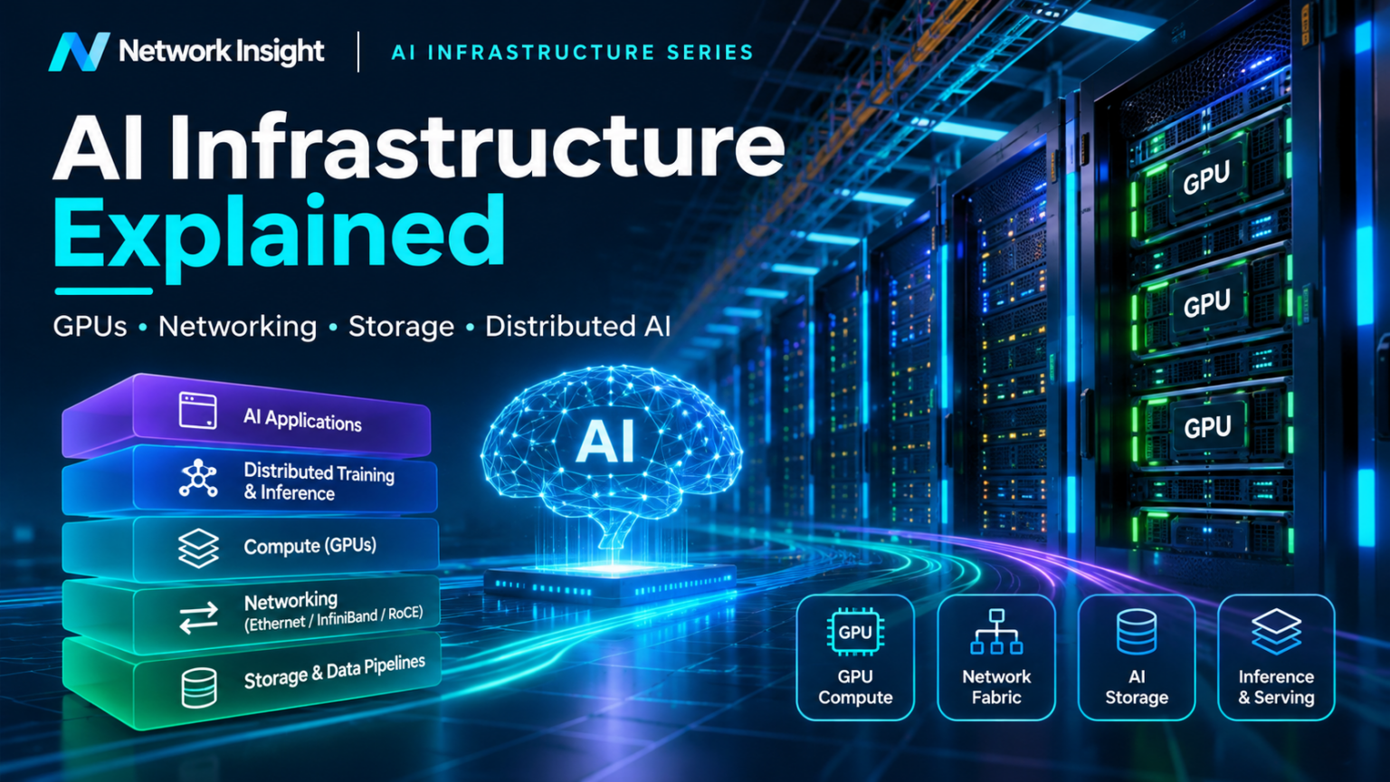
AI Infrastructure Fundamentals: From Traditional Data Centres to AI Computing Platforms
Artificial intelligence introduces a new class of infrastructure requirements. Instead of simply hosting applications, databases, and virtual machines, modern AI platforms must coordinate accelerated computing, high-bandwidth networking, distributed storage, and complex software frameworks to execute demanding training and inference workloads.
Understanding AI infrastructure begins with a fundamental distinction: an AI cluster is not merely a collection of powerful servers. It is a coordinated distributed computing environment in which communication, memory, storage, scheduling, and processing must operate together efficiently.
How AI Infrastructure Differs from Traditional Data Centres
Traditional enterprise data centres support diverse workloads such as web applications, transactional databases, virtual machines, and business services. These systems commonly depend on reliable network connectivity, application availability, predictable latency, and efficient resource sharing.
Their traffic patterns often include client-to-server communication, application-to-database transactions, and east-west communication between distributed services. Although these environments can generate substantial network traffic, many applications do not require tightly synchronized computation across large groups of servers.
AI training environments can behave differently. Distributed training may require hundreds or thousands of accelerators to exchange intermediate results, gradients, or model parameters during repeated computation cycles.
When one accelerator or communication path becomes significantly slower than the others, synchronized operations may have to wait. This makes network congestion, communication efficiency, and accelerator utilization important considerations in overall system performance.
Typically optimized for a broad mixture of application services, virtualization, storage access, and transactional workloads.
Common priorities include availability, flexibility, security, resource efficiency, and predictable application performance.
Designed to coordinate GPU-intensive workloads, high-volume data movement, distributed training, and large-scale model serving.
Important priorities include accelerator utilization, network bandwidth, communication efficiency, memory capacity, and cost per useful computation.
These architectures are not mutually exclusive. AI inference services may run alongside conventional applications, while enterprise data centres can incorporate GPU servers and high-performance networking without becoming dedicated training facilities.
The architectural difference lies primarily in workload behavior and the resulting infrastructure design priorities.
The Six Building Blocks of AI Infrastructure
A production AI platform contains several major infrastructure domains. Understanding the role of each component is essential because performance limitations can emerge at any point in the system.
Accelerated Compute
GPUs and other accelerators execute the mathematical operations required by AI workloads. CPU resources coordinate processing, data preparation, and system-level operations.
High-Performance Networking
Network fabrics connect computing nodes and transport distributed workload traffic. Ethernet, InfiniBand, RDMA, and congestion management technologies can influence communication performance.
Distributed Storage
Storage platforms hold training datasets, model artifacts, checkpoints, and application data. Parallel I/O and caching help supply information at rates required by compute nodes.
Distributed Software
AI frameworks coordinate model execution, parallel computation, gradient synchronization, and communication between accelerators across multiple servers.
Orchestration and Scheduling
Cluster management systems allocate resources, schedule jobs, manage containers, and coordinate the lifecycle of training and inference workloads.
Physical Infrastructure
Power delivery, cooling, rack design, cabling, and physical capacity planning determine how densely accelerator systems can be deployed and operated.
These domains are interdependent. A cluster may have sufficient GPU compute capacity but still perform poorly if storage throughput is inadequate or network congestion delays synchronization between workers.
Engineering Insight
AI infrastructure performance should be evaluated end to end. Purchasing faster accelerators does not automatically improve application throughput if networking, memory, storage, or software coordination remains the limiting factor.
AI Training Versus AI Inference
AI infrastructure supports two major categories of workloads: training and inference. Although both use accelerated computing, their operational characteristics and infrastructure requirements can differ substantially.
During training, a model processes datasets and adjusts its parameters through repeated optimization steps. Large training jobs may distribute computation across multiple GPUs and servers, requiring substantial communication between participating workers.
Inference uses an already trained model to generate predictions, classifications, or responses. Infrastructure must efficiently serve requests while balancing latency, throughput, memory utilization, and cost.
Building and Updating Models
Training workloads repeatedly process data, calculate gradients, and update model parameters. Distributed execution can introduce intensive communication and synchronization requirements.
Serving Model Predictions
Inference workloads process incoming requests using trained models. Serving systems must balance response time, batching efficiency, concurrency, and accelerator memory consumption.
These distinctions are important but not absolute. Large inference deployments can distribute a single model across multiple accelerators, introducing high-bandwidth communication requirements similar to those encountered in distributed training.
Likewise, some training workloads fit within a single accelerator or server and do not require a large network fabric. Infrastructure design must therefore follow the actual workload profile rather than relying on broad labels alone.
Following an AI Workload Through the Infrastructure
To understand the relationship between infrastructure components, consider a distributed training job submitted to an AI computing cluster.
The workload begins with a scheduling decision. The cluster management platform identifies available resources and allocates the required accelerator nodes.
Training data is then supplied through the storage and data pipeline. GPUs execute mathematical operations while the distributed training framework coordinates communication between participating workers.
At appropriate points, the system synchronizes information across accelerators and writes model checkpoints to persistent storage.
This journey demonstrates why AI infrastructure requires coordinated design. The scheduler must allocate suitable resources, storage must supply data efficiently, GPUs must execute computations, and the network must support distributed communication without introducing excessive delays.
Monitoring must also provide visibility into accelerator utilization, communication performance, storage activity, job progress, and infrastructure health. Without this visibility, identifying the source of performance degradation becomes considerably more difficult.
What Makes an AI Infrastructure Architecture Effective?
Successful AI infrastructure design begins with workload requirements. The number of accelerators, model size, parallelization strategy, dataset characteristics, and performance objectives influence every architectural decision.
For distributed training, engineers must consider communication patterns, fabric bandwidth, network oversubscription, congestion behavior, and accelerator placement within the cluster.
For inference, the design may prioritize request latency, model loading, memory capacity, concurrency, batching efficiency, and predictable service availability.
Physical constraints are equally important. High-density accelerator servers can impose substantial power and cooling requirements, while network cabling, transceiver selection, rack placement, and maintenance procedures influence operational complexity.
Ultimately, the objective is to deliver useful workload performance efficiently, rather than optimizing individual infrastructure components in isolation.
Section 1 — Engineering Takeaways
- AI infrastructure is a coordinated distributed computing environment, not simply a collection of GPU servers.
- Traditional data centre principles remain relevant, but AI workloads can introduce more demanding compute and communication characteristics.
- Accelerated compute, networking, storage, distributed software, orchestration, and physical infrastructure must work together.
- Training and inference have different performance objectives and infrastructure requirements.
- End-to-end workload performance is more meaningful than the isolated specifications of individual components.
Inside an AI Infrastructure Platform
Explore how accelerated compute, networking, storage and software platforms combine to support modern AI workloads. Select a layer or simulate a workload journey.
An AI platform is a coordinated system of computing, networking, storage and software services. Each component contributes to the performance and reliability of AI workloads.
Deliver the computing capacity, communication bandwidth, data access and operational controls required by AI applications.
Training vs Inference: Different Infrastructure Demands
Select a workload above to investigate how infrastructure priorities change depending on the execution model.
01 / Model Training
Large-scale computation across GPU clusters. High-throughput data pipelines, accelerator communication and checkpoint storage are critical.
02 / Model Inference
Serving predictions or generated responses. Latency, concurrency, memory capacity, throughput and availability become major design considerations.
GPU Servers and Accelerated Computing: Inside the Compute Architecture of AI Infrastructure
Graphics processing units have become central to modern artificial intelligence because they can execute large numbers of mathematical operations in parallel. However, the performance of an AI computing platform depends on more than GPU processing capability.
CPU coordination, accelerator memory, PCIe connectivity, high-bandwidth GPU interconnects, and server architecture all influence how efficiently AI workloads execute.
Understanding these components is essential for designing AI clusters that can scale beyond a single accelerator or server.
Why GPUs Are Different from Traditional CPUs
Central processing units are designed to execute a broad range of instructions, manage operating systems, coordinate applications, and handle complex control-oriented workloads.
CPUs typically contain a comparatively small number of sophisticated processing cores optimized for low-latency execution, branching logic, and general-purpose computing tasks.
GPUs use a different architectural approach. They contain large numbers of execution resources designed to process many operations concurrently.
This makes GPUs particularly effective for workloads involving matrix multiplication, tensor operations, and other highly parallel calculations commonly found in machine learning and deep neural networks.
Modern AI accelerators also incorporate specialized matrix-processing hardware, such as Tensor Cores, to improve throughput for supported numerical formats and machine learning operations.
CPU — Control and Coordination
Handles operating system functions, application orchestration, data preparation, I/O coordination, and general-purpose processing. CPUs remain essential even in GPU-intensive computing environments.
GPU — Parallel Execution
Executes large volumes of parallel mathematical operations. GPU performance depends on compute resources, memory bandwidth, supported precision formats, and the efficiency of workload execution.
Specialized Matrix Engines
Accelerator architectures may include dedicated matrix-processing units that improve performance for neural network training and inference operations.
Parallel Programming Models
Software platforms such as CUDA and accelerator-aware frameworks coordinate execution across GPU resources and manage data movement between compute and memory domains.
GPU acceleration is most effective when a workload contains sufficient parallelism and can keep the accelerator supplied with data. Serial execution, inefficient memory access, or excessive communication overhead can reduce the expected benefit.
Inside a Multi-GPU AI Server
A modern AI server integrates multiple infrastructure components within a single physical system. These typically include one or more CPUs, system memory, GPU accelerators, local storage, network adapters, and high-speed interconnects.
CPUs coordinate operating system functions and manage many aspects of workload execution. GPUs perform accelerated computation, while dedicated interconnects allow data to move between devices.
Depending on the server architecture, GPUs may communicate through PCIe, dedicated GPU-to-GPU interconnects, or switching fabrics designed for high-bandwidth accelerator communication.
The internal topology of a GPU server matters because not all communication paths provide equivalent performance.
Data transferred between GPUs through a high-bandwidth accelerator fabric may follow a different path from data exchanged between a GPU and host memory through PCIe.
Engineers must therefore understand the relationship between accelerator placement, memory locality, CPU affinity, and interconnect topology when designing distributed workloads.
GPU Memory, HBM, and the Importance of Data Locality
GPU processing performance depends heavily on how quickly data can be supplied to execution resources. A GPU with substantial compute capability may remain underutilized if memory access cannot keep pace with computation.
Many data centre AI accelerators use high-bandwidth memory, or HBM, to provide substantial memory bandwidth close to the GPU processing hardware.
HBM capacity influences how much model state, activation data, and intermediate information can reside directly in accelerator memory.
Memory bandwidth determines how quickly data can move between the accelerator memory subsystem and its processing units. Capacity and bandwidth are therefore separate design considerations.
The closer data resides to the execution resources, the more efficiently many operations can access it. However, different memory tiers offer different trade-offs between capacity, bandwidth, latency, and cost.
When a model exceeds the memory capacity of a single GPU, engineers may distribute model components across multiple accelerators, use memory offloading, or apply techniques that reduce memory requirements.
These approaches introduce additional communication and coordination requirements. Consequently, memory architecture is closely connected to network and interconnect design.
Engineering Insight — Compute Versus Memory
AI workload performance is not determined by accelerator arithmetic throughput alone. Memory capacity, memory bandwidth, data locality, and communication overhead can become the dominant performance constraints.
PCIe, NVLink, and NVSwitch: Moving Data Between GPUs
AI servers require high-speed communication paths between CPUs, GPUs, network adapters, and other devices.
PCI Express, commonly called PCIe, provides a general-purpose high-speed I/O interconnect. It is widely used to connect accelerators, network adapters, and storage devices to host systems.
NVLink is an NVIDIA high-bandwidth interconnect technology designed for communication between supported accelerators and, in certain architectures, between CPUs and GPUs.
NVSwitch extends supported NVLink architectures by providing a switching fabric that enables high-bandwidth communication among multiple GPUs.
| Technology | Primary Role | Engineering Consideration |
|---|---|---|
| PCIe | General-purpose high-speed device connectivity | Link generation, lane width, topology, and shared bandwidth |
| NVLink | High-bandwidth communication between supported processors | Peer connectivity, bandwidth, topology, and device support |
| NVSwitch | Switching fabric for supported multi-GPU NVLink systems | Fabric connectivity, scalability, and collective communication |
| Ethernet / InfiniBand | Communication between computing nodes and networked resources | Network bandwidth, congestion, latency, and transport behavior |
The distinction between intra-node and inter-node communication is particularly important.
Intra-node communication occurs between devices within the same server or accelerator system. Inter-node communication crosses the external network between computing nodes.
Distributed AI frameworks may use both communication domains during a single training workload.
For example, a model may distribute computations across GPUs within one server while synchronizing information with additional servers over a high-performance network fabric.
Scaling from One GPU Server to a Distributed AI Cluster
Consider an illustrative AI infrastructure deployment containing eight compute nodes, each equipped with four GPUs.
This produces a total of 32 accelerators available for distributed workloads. However, the ability to use these GPUs efficiently depends on more than the total accelerator count.
Example — 32-GPU Training Cluster
Each server performs local GPU computation. Distributed training software coordinates operations across all participating nodes. The network fabric transports information exchanged between servers, while storage systems provide training data and checkpoint capacity.
If the workload requires frequent synchronization, the network must support the resulting communication volume without introducing excessive delays.
If the model is divided across multiple GPUs, interconnect bandwidth and accelerator topology may influence the efficiency of model-parallel operations.
If training data cannot be delivered quickly enough, accelerators may spend time waiting rather than performing useful computation.
The engineering objective is therefore to balance compute capacity, memory, communication bandwidth, storage throughput, and workload placement.
Section 2 — Engineering Takeaways
- GPUs accelerate AI workloads through massively parallel computation.
- CPUs remain essential for operating system functions, orchestration, and I/O coordination.
- GPU memory capacity and bandwidth can determine whether workloads execute efficiently.
- PCIe, NVLink, and NVSwitch provide different connectivity capabilities within supported server architectures.
- Intra-node and inter-node communication must both be considered when scaling distributed AI workloads.
- Effective AI infrastructure design requires balancing accelerator performance with communication, storage, and software requirements.
Inside an AI GPU Compute Server
Explore accelerated computing, memory locality, GPU interconnects and distributed AI cluster architecture.
Explore the compute node
A conceptual dual-CPU, four-GPU server. Select a GPU to inspect its role, or launch an animated AI workload.
Each GPU executes massively parallel operations. Its local high-bandwidth memory stores tensors, weights and intermediate data.
AI Memory Hierarchy Explorer
Compare conceptual data placement across GPU HBM, host DRAM and remote storage. Adjust the model working set to observe capacity pressure.
Illustrative single-GPU placement model, not a hardware benchmark. Real frameworks may shard, stream, cache or offload tensors; capacity alone does not predict runtime.
GPU Communication Fabric
Change the interconnect model and see how the communication architecture changes.
NVLink provides high-bandwidth paths between supported GPUs. Actual connectivity and bandwidth depend on the platform generation and topology.
Distributed AI Cluster Builder
Scale a conceptual GPU cluster and examine how compute capacity and network communication requirements grow.
Eight servers provide 32 GPUs. Training across servers introduces inter-node communication, including collective operations such as all-reduce.
Aggregate HBM is the sum of device memory, not a single shared memory pool. GPU memory capacity, NIC count and topology are illustrative design assumptions.
AI Cluster Network Architecture: Designing High-Performance GPU Fabrics
High-performance networking is a foundational component of distributed artificial intelligence. As AI workloads scale beyond individual GPU servers, the network fabric becomes responsible for transporting enormous volumes of data between accelerators, coordinating distributed computation, and maintaining predictable communication performance.
AI cluster networking combines established data centre design principles with demanding requirements for bandwidth, latency, congestion management, and traffic distribution.
Technologies such as leaf-spine architectures, Ethernet, InfiniBand, ECMP, and remote direct memory access provide the foundations for building scalable AI computing environments.
Why AI Workloads Place Different Demands on the Network
Traditional enterprise networks support a diverse mixture of application traffic, client-server communication, database transactions, and distributed services. Network performance is commonly evaluated through availability, throughput, latency, packet loss, and application response times.
Distributed AI training introduces additional communication requirements. When a model is trained across multiple accelerators, participating GPUs may need to exchange gradients, parameters, or intermediate results during repeated computation cycles.
These operations can generate substantial east-west traffic between compute nodes. Some collective communication patterns involve many accelerators exchanging information during coordinated phases of execution.
If network congestion delays communication, participating workers may spend time waiting for synchronization rather than executing useful computation.
High Bandwidth
Distributed training may require substantial aggregate bandwidth between accelerator nodes. Fabric capacity must be designed around workload communication patterns.
Predictable Latency
Communication delays can affect synchronized distributed operations. Tail latency and congestion behavior may be as important as average latency.
Congestion Management
Bursty collective communication can create temporary network hotspots. Queue management, traffic engineering, and transport-level congestion control help manage these conditions.
Scalable Connectivity
AI clusters may expand across racks and network domains. The architecture must provide sufficient path diversity, operational visibility, and capacity for future growth.
The objective is not necessarily to eliminate every microsecond of delay. Instead, engineers must understand the communication characteristics of their workloads and design network capacity and behavior accordingly.
Leaf-Spine Architecture for AI Computing Clusters
Leaf-spine networking is widely used in modern data centres because it provides a scalable topology with predictable path structure and multiple forwarding options between endpoints.
In a conventional two-tier leaf-spine design, compute servers connect to leaf switches. Each leaf switch connects to every spine switch, creating multiple paths between servers attached to different leaf switches.
Traffic between endpoints on different leaves typically traverses a leaf, a spine, and another leaf. Equal-cost multipath routing can distribute eligible flows across available paths.
Leaf-spine architectures offer multiple potential paths between compute nodes. However, the presence of multiple paths does not automatically guarantee balanced traffic distribution.
Flow hashing, traffic entropy, routing design, workload communication patterns, and congestion conditions influence how effectively available bandwidth is used.
Large AI fabrics may also employ additional network tiers, rail-oriented designs, or specialized accelerator networking architectures to meet scaling requirements.
Front-End and Back-End Network Fabrics
AI computing environments frequently distinguish between front-end and back-end network functions.
The front-end network supports management, workload submission, orchestration, storage access, and communication with external services.
The back-end network is commonly designed to support high-performance communication between accelerator nodes during distributed computing operations.
These functions may use physically separate networks, logically isolated fabrics, or shared infrastructure, depending on scale, operational requirements, and architecture.
Application and Platform Connectivity
Provides connectivity for platform services, cluster management, user access, orchestration, and selected storage or data movement functions.
Accelerator Communication
Supports high-bandwidth communication between distributed GPU workers, including collective operations and synchronization traffic.
Network separation can help engineers isolate performance-sensitive traffic, simplify operational policies, and manage different infrastructure requirements independently.
Nevertheless, separation introduces additional cost, cabling, switching, and operational complexity. The appropriate architecture depends on workload scale and business objectives.
Ethernet Versus InfiniBand for AI Networking
Ethernet and InfiniBand are two major networking technologies used in high-performance computing environments. Both can support demanding AI workloads, but they differ in ecosystem, architecture, and operational characteristics.
Ethernet provides a broadly adopted networking foundation with extensive tooling, vendor support, and integration into existing data centre environments.
Ethernet-based AI fabrics may use RoCEv2 to support RDMA communication over IP networks, alongside congestion management mechanisms such as ECN, PFC, and transport-level controls.
InfiniBand is designed for high-performance interconnect environments and provides native RDMA capabilities, fabric management, and specialized communication features.
| Characteristic | Ethernet | InfiniBand |
|---|---|---|
| Primary ecosystem | Enterprise, cloud, and data centre | HPC and accelerated computing |
| RDMA support | RoCE on supported systems | Native RDMA architecture |
| Routing approach | Ethernet/IP fabric mechanisms | InfiniBand fabric forwarding |
| Congestion management | ECN, PFC, transport controls | Fabric-specific mechanisms |
| Operational integration | Broad existing networking ecosystem | Specialized fabric ecosystem |
| Design consideration | Congestion engineering and interoperability | Fabric architecture and platform support |
Neither technology is universally superior. The appropriate choice depends on performance requirements, existing expertise, workload behavior, operational constraints, and the supported hardware ecosystem.
Ethernet-based AI networking is particularly relevant to network engineers familiar with IP routing, ECMP, QoS, telemetry, and data centre fabric design.
Oversubscription, ECMP, and Network Capacity Planning
Network oversubscription describes the relationship between the aggregate bandwidth available to connected endpoints and the bandwidth available toward the rest of the network.
A non-oversubscribed design provides sufficient uplink capacity to match the aggregate downstream capacity at the measured boundary.
Oversubscription can reduce infrastructure cost when workloads do not use all available bandwidth simultaneously. However, aggressive oversubscription may create congestion when distributed AI workloads generate synchronized communication bursts.
Illustrative Leaf Switch Capacity Example
Consider a leaf switch with eight 400 Gb/s server-facing ports and four 400 Gb/s spine-facing uplinks.
If all connected servers simultaneously attempt to transmit at their full port rates toward remote leaves, the uplinks cannot carry the entire offered load without congestion, buffering, or traffic regulation.
This ratio describes aggregate port capacity at the leaf boundary. It does not predict actual application throughput without considering traffic patterns and protocol behavior.
Equal-cost multipath routing allows eligible traffic to use multiple forwarding paths. However, conventional flow-based ECMP can produce uneven utilization when a small number of large flows hash onto the same path.
Flowlet-based techniques, adaptive routing, and other load-distribution approaches may improve utilization on supported platforms, but they introduce additional design and operational considerations.
Engineering Insight — Bandwidth Is Not Enough
A network fabric can have substantial aggregate bandwidth and still experience localized congestion. Effective AI networking requires understanding traffic placement, flow distribution, queue behavior, and synchronization patterns across the cluster.
Engineering a Network Fabric for a 32-GPU Cluster
Consider the 32-GPU example introduced in the previous section: eight servers, each containing four accelerators.
Suppose each server has a dedicated 400 Gb/s connection to a back-end network fabric. The aggregate server-facing bandwidth is therefore 3.2 Tb/s, measured as the sum of the eight nominal link rates.
This does not mean that every workload will achieve 3.2 Tb/s of useful application throughput. Actual performance depends on communication patterns, protocol overhead, endpoint capability, network topology, and congestion.
Engineers must decide how to distribute servers across leaf switches, how many uplinks each leaf requires, and whether the fabric should be designed for minimal oversubscription.
They must also consider failure domains, redundant connectivity, network telemetry, and the impact of maintenance or link failures on distributed jobs.
For communication-intensive training, the network may be designed with greater bandwidth headroom and closer attention to accelerator placement and traffic locality.
For workloads with lower communication requirements, a more economical design may be sufficient.
Section 3 — Engineering Takeaways
- Distributed AI workloads can generate intensive east-west communication between accelerator nodes.
- Leaf-spine architectures provide scalable connectivity and multiple forwarding paths between compute nodes.
- Front-end and back-end network functions may be separated to manage different traffic requirements.
- Ethernet and InfiniBand both support high-performance AI networking, with different architectural and operational characteristics.
- Oversubscription, ECMP behavior, congestion management, and workload placement influence effective network performance.
- AI fabric design should be driven by actual workload communication requirements rather than bandwidth specifications alone.
Inside the AI Networking Fabric
Investigate how GPU clusters communicate across a leaf-spine fabric. Simulate distributed training traffic, observe congestion, and examine network resilience.
The spine layer provides paths between leaf switches. GPU servers connect through leaves, while multiple spine paths support load distribution and resilience.
Bandwidth, latency, topology, congestion control and distributed communication.
Network Investigation Dashboard
Illustrative scenario metrics, not measurements from a physical network.
Educational model: six GPU endpoints and a two-spine, three-leaf Clos-style fabric. The animations represent logical communication paths. Utilization and congestion values are illustrative scenario assumptions, not results of a packet-level or RDMA simulation. All-reduce is represented through selected peer exchanges rather than a complete collective algorithm.
RDMA, RoCEv2 and High-Performance Networking: Inside the Transport Architecture of AI Clusters
Distributed AI workloads depend on efficient communication between computing nodes. When thousands of accelerators exchange gradients, parameters, and intermediate results, conventional network connectivity alone is not sufficient to guarantee predictable performance.
Remote Direct Memory Access, or RDMA, provides a communication model designed to reduce CPU involvement and enable efficient data transfers between registered memory regions.
RoCEv2 extends RDMA communication into routable Ethernet/IP environments, making it an important technology in modern AI networking architectures.
Why RDMA Matters for Distributed AI
Traditional network applications commonly use socket-based communication over TCP/IP. The operating system networking stack manages transport functions, buffering, protocol processing, and application data delivery.
This architecture provides flexibility, reliability, and broad interoperability. However, conventional socket-based communication can introduce CPU overhead, memory copying, and software processing costs that may become significant in high-throughput computing environments.
RDMA provides a different communication model. Supported network adapters can transfer data directly between registered memory regions with reduced involvement from the remote CPU during the data path.
RDMA does not eliminate all CPU processing, nor does it guarantee zero-copy behavior for every application or system configuration. Applications must still establish resources, register memory, manage permissions, and coordinate communication.
Conceptual software path. Modern socket implementations may use hardware offloads and zero-copy optimizations.
Conceptual one-sided RDMA data path. Setup, authorization, completion handling, and application coordination remain necessary.
RDMA is particularly valuable when applications need to move substantial amounts of data efficiently between computing nodes.
Distributed AI frameworks may use RDMA-capable communication libraries to exchange tensors and coordinate collective operations across multiple servers.
Queue Pairs, Memory Registration, and RDMA Operations
RDMA communication relies on several important resources, including queue pairs, completion queues, and registered memory regions.
A queue pair typically contains a send queue and a receive queue. Applications post work requests that describe communication operations for the RDMA adapter to execute.
Memory registration allows the adapter to access specific memory regions under defined permissions. Access keys help control local and remote memory operations.
RDMA Write
Allows a requester to write data into an authorized remote memory region. The remote application does not need to process each incoming data transfer directly.
RDMA Read
Allows a requester to retrieve data from an authorized remote memory region, subject to transport capabilities and configured permissions.
Send / Receive
Uses message-oriented communication where receive buffers are posted by the receiving side. This differs from one-sided RDMA Read and Write operations.
Completion Queues
Provide completion information for supported work requests. Applications use completions to track communication progress and identify operation errors.
RDMA transport behavior also depends on the selected queue pair type. Reliable Connected transport, commonly abbreviated RC, provides reliable, ordered communication semantics for supported operations.
Other transport types have different capabilities and reliability properties. Understanding these distinctions is important when troubleshooting communication behavior.
Understanding RoCEv2 Packet Structure
RDMA over Converged Ethernet version 2, or RoCEv2, enables RDMA traffic to traverse routable IP networks.
RoCEv2 encapsulates RDMA transport information inside UDP/IP packets, allowing compatible networking infrastructure to forward traffic across Layer 3 boundaries.
The UDP destination port commonly associated with RoCEv2 is 4791. The IP header also enables mechanisms such as Explicit Congestion Notification, or ECN, to signal network congestion.
The Base Transport Header contains information used by the RDMA transport, including operation identification and queue pair-related fields.
Additional transport headers may carry addressing or operation-specific information. For example, certain RDMA operations require remote memory addressing and access keys.
From a network engineering perspective, RoCEv2 introduces the challenge of transporting latency-sensitive, high-throughput RDMA traffic across a packet-switched Ethernet/IP fabric.
ECN, PFC, and DCQCN in AI Network Fabrics
AI workloads can generate bursts of traffic when multiple accelerators communicate during synchronized operations.
If incoming traffic exceeds the forwarding capacity of a switch egress port, packets may accumulate in output queues.
Without effective congestion management, queues can grow, latency can increase, and packets may eventually be dropped.
Ethernet-based RoCE deployments commonly use several complementary mechanisms to manage congestion and reduce disruptive packet loss.
| Mechanism | Function | Engineering Consideration |
|---|---|---|
| ECN | Marks ECN-capable packets to indicate congestion without necessarily dropping them. | Queue thresholds and endpoint response behavior. |
| PFC | Applies link-level pause to selected traffic priorities. | Head-of-line blocking, pause propagation, and deadlock risks. |
| DCQCN | Endpoint congestion control that uses congestion feedback to adjust RoCE sending rates. | Rate adaptation, stability, and compatibility with network configuration. |
| ECMP | Distributes eligible flows across multiple forwarding paths. | Flow collisions, traffic polarization, and uneven utilization. |
ECN allows a congested switch to mark packets instead of immediately discarding them, provided the packets are ECN-capable and the network is configured appropriately.
In a common DCQCN feedback sequence, congestion-marked packets reach the receiver, which generates Congestion Notification Packets, or CNPs, toward the sender.
The sender's rate-control mechanism then adjusts transmission behavior in response to congestion feedback.
Priority Flow Control, or PFC, operates differently. It allows a device to pause transmission for selected Ethernet priorities when configured thresholds are reached.
Although PFC can help prevent packet loss under certain conditions, excessive pause propagation can introduce head-of-line blocking and broader performance problems.
Consequently, PFC should not be treated as a substitute for effective end-to-end congestion control.
Engineering Insight — Lossless Does Not Mean Congestion-Free
A fabric engineered to minimize packet loss can still suffer from congestion, queueing delays, pause storms, and unfair bandwidth allocation. Effective RoCE performance requires coordinated switch configuration, endpoint congestion control, and telemetry.
Investigating a RoCEv2 Congestion Incident
Consider a distributed AI training workload operating across multiple GPU servers connected through a leaf-spine Ethernet fabric.
During synchronized communication, several senders transmit toward a shared destination. The resulting traffic burst causes increased queue occupancy on a particular leaf switch egress port.
The cluster begins to experience longer synchronization times, even though the GPUs themselves remain operational.
AI Training Job — Network Congestion Investigation
The investigation should examine whether congestion is localized to a particular path, whether traffic is unevenly distributed across ECMP links, and whether endpoint congestion feedback is functioning correctly.
Engineers should also inspect PFC pause counters, queue occupancy, packet drops, ECN marking statistics, CNP activity, and application-level performance.
A high ECN marking rate is not automatically evidence of a configuration failure. ECN may be functioning correctly by signaling congestion before packet loss occurs.
Similarly, PFC activity does not always indicate a fault. The concern arises when pause behavior becomes excessive, persistent, or disruptive to unrelated traffic.
Effective troubleshooting requires correlating network telemetry with workload behavior. Engineers must determine whether the root cause is insufficient capacity, traffic imbalance, congestion-control configuration, or the communication pattern generated by the application.
Section 4 — Engineering Takeaways
- RDMA enables efficient communication between registered memory regions with reduced CPU involvement in supported data paths.
- Queue pairs, completion queues, memory registration, and access permissions are fundamental RDMA concepts.
- RoCEv2 encapsulates RDMA transport information over UDP/IP, enabling routable Ethernet-based deployments.
- ECN, PFC, and DCQCN perform different but complementary congestion-management functions.
- PFC can introduce operational risks when pause behavior propagates excessively.
- RoCE troubleshooting requires correlating switch telemetry, endpoint feedback, and distributed workload performance.
RDMA & RoCEv2 Network Engineering Lab
Trace GPU traffic, inspect transport headers, control congestion and troubleshoot an AI training fabric.
GPU-to-GPU RDMA Communication
Follow a conceptual RDMA WRITE operation across two AI compute servers and an Ethernet switching fabric.
Start the transfer to examine memory registration, work queues, RNIC processing, network forwarding and remote memory placement.
Conceptual operation: assumes a pre-established reliable-connected queue pair and correctly registered, authorized destination memory. GPU-direct paths require supported hardware and software.
Inside a RoCEv2 Packet
Select each header to examine how RDMA transport is carried across a routable IP network.
The Ethernet header carries source and destination MAC addresses and may contain VLAN tagging. The frame is forwarded to the next hop at Layer 2.
Simplified RDMA WRITE Only/First-style view. Exact headers depend on opcode, IP version, VLAN configuration and segmentation. Additional headers, padding, ICRC and Ethernet FCS are not all drawn separately.
RoCEv2 Congestion Control Simulator
Change offered traffic and experiment with ECN marking, priority flow control and simplified DCQCN-style sender adaptation.
Switch egress queue occupancy
Queue occupancy history
The model tracks queue buildup and simplified congestion feedback over discrete time steps.
Educational discrete-time model, not a standards-compliant DCQCN implementation. ECN marks traffic, PFC can pause upstream priority traffic, and DCQCN uses congestion feedback to adjust sender rate. Thresholds and rate changes here are illustrative.
AI Training Fabric · Incident Investigation
A distributed training job experiences unpredictable iteration times during a high-volume gradient exchange.
Multiple GPU workers converge on one oversubscribed egress port. Queue occupancy increases, ECN marks appear, and the training job experiences communication delays.
Incident evidence
Switch telemetry: sustained queue growth, ECN marking and occasional drops. Endpoint telemetry: elevated collective operation completion time.
Select engineering responses
Select the actions you would take to stabilize the training network.
Distributed AI Training: Parallelism, Collective Communication, and GPU Synchronization
Training large artificial intelligence models frequently requires more compute capacity and memory than a single accelerator can provide. Distributed training addresses this challenge by dividing computation, model state, or training data across multiple GPUs and computing nodes.
However, scaling a workload across additional accelerators introduces communication and synchronization requirements that can significantly influence training efficiency.
Understanding data parallelism, tensor parallelism, pipeline parallelism, and collective communication is essential for designing infrastructure that can support large-scale AI training.
Why AI Training Must Be Distributed
Modern AI models can contain billions of parameters, requiring substantial computational resources and memory capacity during training.
Training involves repeatedly processing data, calculating predictions, evaluating errors, computing gradients, and updating model parameters.
The memory required for training includes more than model parameters. Activations, gradients, optimizer states, temporary buffers, and communication resources can consume significant accelerator memory.
When a workload exceeds the capacity of a single GPU, distributed training allows multiple accelerators to cooperate on the same computation.
The challenge is deciding how to distribute the workload while minimizing communication overhead and maintaining efficient accelerator utilization.
Engineering Principle
Adding GPUs does not guarantee proportional improvements in training throughput. Communication, synchronization, memory access, workload imbalance, and software overhead can limit scaling efficiency.
Data Parallelism, Tensor Parallelism, and Pipeline Parallelism
Distributed AI frameworks use several parallelization strategies to divide training workloads across accelerators.
These strategies differ in how computation and model state are distributed, and each creates different communication patterns.
Data Parallelism
Each worker processes a different portion of training data using a model replica. Gradients are synchronized so participating workers can maintain consistent model updates.
Tensor Parallelism
Individual tensor operations or model components are divided across multiple accelerators. Participating GPUs exchange intermediate results during model execution.
Pipeline Parallelism
Different portions of the model execute on separate accelerators. Microbatches can move through pipeline stages to improve utilization and overlap work.
Data parallelism is often effective when model replicas fit within accelerator memory and training can be divided across independent data batches.
Tensor parallelism is useful when individual model operations or layers must be distributed across multiple devices. It can introduce frequent communication between accelerators.
Pipeline parallelism divides model execution into stages. Its efficiency depends on stage balance, microbatch scheduling, and communication between pipeline boundaries.
Large-scale systems frequently combine multiple strategies. For example, tensor parallelism may operate within a server, while data parallelism spans multiple servers across the network fabric.
Understanding AllReduce and GPU Synchronization
Distributed training requires participating workers to exchange information during computation. Collective communication operations coordinate these exchanges across groups of accelerators.
Common collective operations include AllReduce, AllGather, ReduceScatter, Broadcast, and point-to-point communication between workers.
AllReduce is particularly important in synchronous data-parallel training. It combines values from participating workers using a reduction operation and makes the resulting values available to every participant.
For example, workers may calculate gradients independently and then use AllReduce to obtain the combined gradients required for consistent model updates.
+
AllGather
In a ring-based AllReduce algorithm, participating workers exchange chunks of data with neighboring workers through repeated steps.
During ReduceScatter, workers combine contributions so that each participant obtains a reduced portion of the data.
During AllGather, the reduced portions are distributed until every worker possesses the complete reduced result.
Communication libraries such as NVIDIA NCCL can select different collective algorithms and communication paths based on hardware topology, message size, and runtime configuration.
| Operation | Purpose | Typical AI Use |
|---|---|---|
| AllReduce | Reduce values and distribute the result to all participants. | Gradient synchronization in data-parallel training. |
| AllGather | Collect distributed data portions at every participant. | Reconstructing sharded tensors or parameters. |
| ReduceScatter | Reduce distributed values and scatter portions of the result. | Sharded gradient processing and collective algorithms. |
| Broadcast | Distribute data from one participant to others. | Model state distribution and initialization. |
| Point-to-Point | Exchange data between selected workers. | Pipeline stage communication and activation transfer. |
Collective communication can generate substantial network traffic. The impact depends on tensor sizes, collective algorithms, worker placement, network bandwidth, and accelerator interconnect topology.
Following a Distributed Training Step
To understand how distributed training affects infrastructure, consider a synchronous data-parallel training step.
Each worker receives a portion of the training data and performs a forward pass through its local model replica.
The backward pass calculates gradients, which are then synchronized across workers before model parameters are updated consistently.
The synchronization phase creates an important dependency between computation and network communication.
If one worker experiences slower computation or communication, other workers may be delayed at synchronization points.
Consequently, distributed training performance depends on both accelerator efficiency and communication consistency across the cluster.
Estimating AllReduce Communication Cost
Collective communication introduces data movement that must be considered during network capacity planning.
For a simple ring AllReduce with N participating workers and a message containing S bytes, the approximate data transferred per worker across both phases is:
Illustrative Ring AllReduce Calculation
= 2 × 7 / 8 × 1 GB
= 1.75 GB
This simplified estimate assumes an ideal ring AllReduce algorithm with evenly divided data chunks. It represents the approximate total data sent by each worker, not the aggregate bytes across the entire cluster.
Actual execution time depends on bandwidth, communication latency, protocol overhead, topology, contention, and implementation details.
The calculation illustrates why collective communication can place substantial demands on AI network fabrics.
However, communication volume alone does not determine training performance. The ability to overlap communication with computation and distribute traffic efficiently can significantly influence results.
Troubleshooting Poor GPU Scaling Efficiency
Consider a distributed training job that performs efficiently on four GPUs but experiences disappointing throughput improvements when expanded to sixteen GPUs.
The GPUs are operational, network connectivity is established, and the training application completes successfully.
Nevertheless, synchronization delays increase as additional workers participate.
Distributed Training — Scaling Investigation
The investigation should begin by comparing compute time, collective communication time, data loading performance, and synchronization delays across participating workers.
Engineers should examine network link utilization, ECMP distribution, congestion indicators, RDMA performance, GPU placement, and interconnect topology.
It is also important to determine whether one worker consistently operates more slowly than the others, creating a synchronization bottleneck.
Poor scaling does not automatically indicate a network fault. The cause may be insufficient workload parallelism, inefficient collective algorithms, small batch sizes, imbalanced pipeline stages, or storage delays.
A useful investigation correlates GPU profiling data, framework communication traces, network telemetry, and application-level training throughput.
Section 5 — Engineering Takeaways
- Distributed training divides model computation, data, or model state across multiple accelerators.
- Data parallelism, tensor parallelism, and pipeline parallelism create different communication patterns.
- Collective operations such as AllReduce and AllGather coordinate data exchange between distributed workers.
- Ring AllReduce can be modeled as ReduceScatter followed by AllGather.
- Synchronization overhead, communication topology, and workload imbalance influence scaling efficiency.
- Effective troubleshooting requires correlating compute, communication, storage, and application behavior.
AI Workload Orchestration & GPU Scheduling
Explore how an AI platform allocates accelerators, schedules training and inference workloads, manages contention, and responds to infrastructure failures.
No workloads submitted.
AI platforms coordinate accelerator allocation, workload placement and resource availability. Scheduling policies determine which jobs run and which remain queued.
Resource requests, GPU availability, scheduling constraints and workload placement.
Cluster Operations Dashboard
Observe how submitted jobs affect accelerator allocation and scheduler decisions.
Scheduler Event Timeline
Educational scheduler model. Each training job requests four GPUs on one node; each inference job requests one GPU. Jobs run until reset or node failure. Placement is first-fit with whole-GPU allocation. The simulation does not implement Kubernetes, actual GPU execution, preemption, checkpoint restoration, or real scheduling performance measurements.
AI Storage and Data Pipelines: Feeding GPUs, Distributed Storage, and Checkpoint Performance
High-performance GPUs and network fabrics are only part of an effective AI computing environment. Training and inference workloads also depend on storage systems capable of delivering data at sufficient throughput, supporting concurrent access, and maintaining reliable model state.
If data cannot be supplied quickly enough, expensive accelerators may spend time waiting for input rather than performing useful computation.
AI infrastructure therefore requires coordinated design across storage, networking, data processing, memory, and accelerator resources.
Understanding the AI Data Pipeline
AI training begins with data. Depending on the workload, this may include text, images, video, audio, structured records, or large collections of preprocessed training samples.
Before this information reaches the GPU, it may pass through several infrastructure components, including object storage, distributed file systems, preprocessing services, local caches, and host memory.
Each stage introduces potential throughput, latency, and resource constraints.
Efficient pipelines attempt to overlap data loading and preprocessing with GPU execution.
Techniques such as prefetching, parallel workers, caching, batching, and asynchronous transfers can help reduce accelerator idle time.
However, increasing the number of data-loading workers does not automatically improve performance. Excessive concurrency may overload storage systems, consume CPU resources, or create network contention.
Storage Tiers in an AI Computing Environment
AI platforms frequently use multiple storage tiers because no single technology is ideal for every workload requirement.
Capacity-oriented storage provides a repository for large datasets and model artifacts, while higher-performance storage supports active training and repeated data access.
Local NVMe Storage
High-performance SSDs attached to compute servers can provide low-latency access to cached datasets, temporary files, and selected workload data.
Local storage can reduce repeated network transfers, but capacity and data placement must be managed across nodes.
Distributed File Systems
Parallel or distributed file systems can provide shared access to datasets across multiple compute nodes.
Performance depends on storage architecture, metadata operations, client concurrency, network capacity, and workload access patterns.
Object Storage
Object storage provides scalable repositories for datasets, model artifacts, and checkpoints.
It is well suited to large-scale capacity needs, although access characteristics differ from traditional file-system semantics.
A common architecture stages frequently accessed data from capacity-oriented storage into a higher-performance shared or local tier.
The appropriate design depends on dataset size, access frequency, concurrency, recovery requirements, and the available budget.
Parallel File Systems and High-Concurrency Data Access
Distributed training may involve hundreds or thousands of workers accessing large datasets. Storage systems must support concurrent requests without introducing excessive delays.
Parallel file systems such as Lustre and IBM Storage Scale are examples of technologies used in high-performance computing environments.
These systems distribute storage responsibilities across multiple components, allowing data access to scale beyond the capabilities of a single storage server.
However, parallelism introduces additional engineering concerns. Small-file workloads, metadata contention, uneven data placement, and insufficient client-side concurrency can limit throughput.
Aggregate Throughput
Storage bandwidth must support the combined demand of participating training workers, not merely the performance of an individual client.
Metadata Performance
Large numbers of file opens, directory lookups, and metadata operations can become bottlenecks, particularly with many small training files.
Data Locality
Caching and staging frequently accessed data closer to compute resources can reduce repeated network transfers and improve predictability.
Network Capacity
Storage performance depends on the network connecting clients to storage services. Congestion and oversubscription can limit effective data delivery.
AI storage performance should therefore be evaluated using representative application access patterns rather than relying exclusively on sequential bandwidth benchmarks.
GPU Starvation: When Storage Becomes the Bottleneck
GPU starvation occurs when accelerators cannot receive sufficient work or data to remain productively occupied.
Although storage is one possible cause, GPU idle time may also result from CPU preprocessing, synchronization delays, application scheduling, or inefficient workloads.
Consider an AI training environment where storage throughput is insufficient to sustain the required batch delivery rate.
The immediate symptom may appear as low GPU utilization, but the root cause could exist several layers away from the accelerator.
Engineers should compare data-loader wait time, storage latency, storage throughput, CPU utilization, network performance, and GPU execution timelines.
This correlation helps distinguish storage bottlenecks from preprocessing limitations or synchronization delays.
Engineering Insight — Follow the Data
When GPUs are idle, investigate the complete data path rather than immediately increasing accelerator capacity. A faster GPU cannot compensate for a pipeline that consistently fails to supply training data.
Model Checkpointing and Storage Bandwidth
Long-running training jobs must protect progress against hardware failures, software errors, interruptions, and planned maintenance.
Checkpointing periodically saves sufficient model and training state to allow a workload to resume.
Depending on the framework and configuration, checkpoints may contain model parameters, optimizer state, scheduler information, and other training metadata.
Large distributed models can generate substantial checkpoint data, creating short periods of intensive storage and network activity.
Illustrative Checkpoint Bandwidth Calculation
Consider a distributed training job that must save a 2 TB checkpoint within a five-minute window.
≈ 6.67 GB/s
≈ 53.3 Gb/s
This calculation uses decimal units and represents the minimum sustained logical data write rate.
Real systems require additional headroom for protocol overhead, metadata operations, storage contention, redundancy, and variations in effective throughput.
Checkpoint design involves tradeoffs between checkpoint frequency, storage consumption, application interruption, and potential work lost after a failure.
Techniques such as asynchronous checkpointing, incremental checkpoints, and sharded state storage may reduce disruption, depending on framework capabilities.
Troubleshooting a Storage Bottleneck in an AI Cluster
Consider a distributed training workload operating across several GPU servers.
The network fabric is healthy, GPU temperatures are normal, and the application has sufficient accelerator memory.
Nevertheless, training throughput remains below expectations. GPU activity alternates between computation and prolonged idle periods.
AI Training Job — Storage Pipeline Investigation
The investigation should begin by identifying where training workers spend time waiting. Application profiling may reveal that data-loading operations consume a significant portion of each training step.
Engineers should inspect storage throughput, request latency, metadata activity, cache hit rates, network utilization, and CPU preprocessing performance.
The objective is to determine whether the bottleneck originates in storage, the network path, data transformation, or application-level pipeline configuration.
Potential improvements may include dataset sharding, caching, prefetching, larger sequential reads, additional data-loader parallelism, or changes to storage architecture.
Each change should be validated using measured application performance. Improving a storage benchmark does not necessarily improve end-to-end training throughput.
| Observed Symptom | Possible Cause | Investigation |
|---|---|---|
| Low GPU activity | Input pipeline cannot deliver batches quickly enough. | Compare GPU timelines with data-loader wait time. |
| High metadata latency | Excessive small-file operations or metadata contention. | Inspect file access patterns and metadata service metrics. |
| Uneven storage throughput | Data placement imbalance, client contention, or network congestion. | Correlate per-client throughput and network telemetry. |
| Long checkpoint pauses | Insufficient write bandwidth or synchronous checkpoint overhead. | Measure checkpoint duration, write throughput, and job stalls. |
Section 6 — Engineering Takeaways
- AI training performance depends on efficient movement of data from storage into accelerator memory.
- Local NVMe, distributed file systems, and object storage serve different performance and capacity requirements.
- Parallel storage performance depends on concurrency, metadata behavior, network capacity, and application access patterns.
- GPU starvation can result from storage, preprocessing, synchronization, or scheduling bottlenecks.
- Checkpointing introduces substantial storage and network bandwidth requirements for large distributed models.
- Effective troubleshooting requires correlating storage, network, CPU, GPU, and application telemetry.
AI Storage & Data Pipeline Investigation Lab
Explore the journey from distributed storage to GPU memory. Investigate starvation, throughput constraints and checkpoint performance.
Inside the AI Training Data Pipeline
Follow training data through a simplified four-stage architecture. Select any component to inspect its engineering responsibilities.
Start the data journey or select a component to inspect how training data reaches the GPU.
GPU Starvation & Throughput Simulator
Configure three independent capacities. The slowest stage limits the sustainable delivery of training data.
Estimated GPU data-feed efficiency
The storage system cannot supply training data at the rate demanded by the GPUs.
Illustrative steady-state throughput model. Data-feed efficiency is not measured GPU utilization. Real systems also depend on caching, prefetching, batch size, computation time and I/O overlap.
AI Model Checkpointing Simulator
Explore how checkpoint size and effective write bandwidth influence training interruptions.
Checkpoint write progress
Checkpointing protects training progress, but large synchronous writes can interrupt compute operations and increase storage pressure.
Assumes a blocking checkpoint every configured number of minutes of active training, with no overlapping I/O, compression or additional serialization overhead. Animation time is compressed.
Storage Incident · GPU Training Slowdown
A large AI training job has slowed despite healthy GPU hardware and a functioning compute network.
During peak training hours, multiple jobs read datasets from the same storage tier. GPU workers repeatedly wait for the next training batch.
Observed telemetry
Read throughput history
Select your corrective actions
Review the evidence and choose the actions most likely to address the training slowdown.
AI Inference Infrastructure: Model Serving, Request Routing, KV Cache, and GPU Performance
AI training creates the model. Inference infrastructure makes that model available to users, applications, and services. Production inference systems must deliver responses with predictable latency while efficiently sharing expensive accelerator resources across concurrent requests.
Unlike training, which focuses primarily on optimizing model parameters, inference focuses on executing a trained model to generate predictions, classifications, embeddings, or new content.
The infrastructure challenge is balancing response time, throughput, GPU memory, concurrency, availability, and operational cost.
Following an AI Inference Request
A production inference request typically passes through several infrastructure layers before reaching the accelerator executing the model.
These layers may include API gateways, authentication, traffic routing, request queues, inference schedulers, model-serving processes, and accelerator resources.
The response may then be returned as a complete result or streamed incrementally to the requesting application.
The request path introduces multiple potential bottlenecks. Queueing delays may occur before the GPU begins processing, while model execution itself depends on accelerator capacity, memory availability, and scheduling behavior.
Network engineers must also consider the connectivity between gateways, model servers, storage services, and distributed accelerator nodes.
Prefill and Decode in Large Language Model Inference
Autoregressive language-model inference is commonly divided into two major execution phases: prefill and decode.
During prefill, the model processes the input prompt and prepares the attention state required for subsequent token generation.
During decode, the model generates output tokens incrementally, using previously computed attention information.
Processing the Input Prompt
The model processes the prompt tokens and creates the attention state used for subsequent generation.
Prefill performance is influenced by prompt length, model architecture, compute throughput, and memory behavior.
Generating Output Tokens
The model generates output tokens sequentially, updating the attention state as the sequence grows.
Decode performance can be sensitive to memory bandwidth, KV-cache size, batch composition, and accelerator utilization.
These phases create different performance characteristics. Prefill often benefits from substantial parallel computation, while decode can become constrained by memory movement and per-token execution overhead.
Some advanced serving architectures separate prefill and decode workloads across different accelerator resources to optimize scheduling and capacity.
Dynamic and Continuous Batching
GPU inference becomes more economical when multiple requests can share accelerator resources efficiently.
Batching combines work from multiple requests so the model server can execute compatible operations together.
Static batching waits for a group of requests to be assembled before processing begins. This can improve throughput but may introduce queueing delays.
Continuous batching allows the serving system to update the active request set between generation iterations, admitting new requests as capacity becomes available.
Continuous batching can improve accelerator utilization by reducing idle capacity between request groups.
However, larger active batches increase memory consumption and may affect per-request latency.
Production systems must balance batch size, queueing delay, available KV-cache memory, token throughput, and service-level objectives.
KV Cache and GPU Memory Management
During transformer-based autoregressive inference, attention mechanisms use key and value tensors associated with previously processed tokens.
The KV cache stores this information so the model does not need to recompute the same attention state from scratch at every generation step.
KV-cache memory usage depends on model architecture, number of layers, key/value heads, head dimensions, data precision, sequence length, and concurrent requests.
Long prompts and many simultaneous requests can significantly increase memory pressure.
When memory becomes constrained, the serving system may need to limit concurrent requests, reduce batch sizes, evict cached state, or use supported offloading strategies.
Techniques such as paged KV-cache management can reduce memory fragmentation and improve allocation efficiency in supported inference engines.
Engineering Insight — GPU Memory Is a Scheduling Resource
In production inference, available GPU memory influences how many requests can execute concurrently. Capacity planning must consider model weights, KV-cache growth, temporary buffers, and workload variability.
Latency, Throughput, and Inference Capacity Planning
Inference systems are commonly evaluated using several performance metrics.
Time to First Token, or TTFT, measures the elapsed time between request initiation and the first generated output token becoming available to the client.
Time per Output Token, often measured as inter-token latency, describes the rate at which additional tokens are generated.
End-to-end latency includes the complete request lifecycle, including routing, queueing, execution, and response delivery.
| Metric | Meaning | Engineering Importance |
|---|---|---|
| TTFT | Time until the first output token is delivered. | Interactive responsiveness and initial queueing delays. |
| Inter-Token Latency | Time between successive output tokens. | Streaming response smoothness and decode performance. |
| Tokens per Second | Output token generation rate for a request or the serving system. | Throughput and capacity efficiency. |
| Concurrent Requests | Number of requests being served simultaneously. | Scheduler behavior and memory requirements. |
| P95 / P99 Latency | Response-time percentiles across requests. | Tail performance and service reliability. |
Illustrative Inference Response Calculation
Consider a request with a time to first token of 400 milliseconds. The model then generates a total of 100 output tokens with an average interval of 25 milliseconds between successive tokens.
= 2.875 seconds
This simplified calculation assumes the first token is included in TTFT and the remaining 99 tokens are generated at a constant average interval.
Actual latency varies with queueing, batching, prompt length, output length, network conditions, and server scheduling.
Increasing batch size may improve aggregate throughput while also increasing latency for individual requests.
Production inference requires selecting an operating point that satisfies both performance objectives and infrastructure cost constraints.
Scaling and Troubleshooting Production Inference
Production inference platforms must handle changing request rates, variable prompt lengths, different model sizes, and occasional infrastructure failures.
Scaling strategies may include adding model replicas, increasing accelerator capacity, adjusting batching policies, and routing requests across multiple serving nodes.
Autoscaling decisions should consider queue depth, request arrival rate, token throughput, latency objectives, and the time required to initialize new model-serving instances.
Request Routing
Distribute requests across healthy model replicas while accounting for capacity, model availability, and workload characteristics.
Autoscaling
Adjust serving capacity using workload-aware metrics rather than relying exclusively on generic CPU utilization.
Observability
Monitor TTFT, token throughput, queue latency, GPU memory, cache occupancy, and request failures.
Availability
Design for replica failures, model-loading delays, network faults, and capacity loss during maintenance.
Troubleshooting inference requires distinguishing application-level delays from scheduler, accelerator, memory, and network bottlenecks.
Production AI Service — Rising Response Latency
During a traffic increase, the inference service begins experiencing longer response times. Requests accumulate in the scheduler queue, while GPU memory approaches its configured capacity.
The investigation should compare request arrival rates, active batch sizes, queueing delays, prefill time, decode throughput, and memory occupancy.
Engineers should also determine whether the slowdown affects every model replica or only a subset of serving nodes.
Potential causes include insufficient serving capacity, excessive request concurrency, long-context workloads, inefficient batching, model-loading delays, or network-related failures.
The correct remediation depends on identifying which stage of the request lifecycle is responsible for the delay.
Section 7 — Engineering Takeaways
- Inference infrastructure serves trained models to applications and users.
- Production request paths commonly involve gateways, schedulers, model servers, and accelerator resources.
- Prefill and decode have different compute and memory characteristics.
- Continuous batching improves scheduling flexibility but introduces latency and memory tradeoffs.
- KV-cache capacity is a major constraint on concurrent language-model inference.
- Effective operations require monitoring TTFT, token throughput, queue depth, memory pressure, and tail latency.
AI Infrastructure Incident Investigation
Investigate operational failures across GPU compute, networking, storage and distributed training. Analyze telemetry, identify the root cause and apply the appropriate corrective action.
Root Cause Investigation
Select the most likely cause using the available incident evidence.
Identify the correct root cause before applying remediation.
Incident Event Timeline
Educational incident scenarios with illustrative telemetry. Each scenario is constructed around a specific root cause. The widget does not collect live infrastructure metrics or execute changes against a real cluster. Real incident diagnosis requires additional evidence and validation.
AI Infrastructure Security and Operations: Zero Trust, GPU Isolation, Observability, Power, Cooling, and Reliability
AI infrastructure must do more than execute workloads efficiently. Production environments require security controls, operational visibility, reliable resource allocation, and physical infrastructure capable of supporting sustained high-density computing.
Large AI clusters combine valuable training datasets, proprietary models, high-performance accelerators, distributed software, and complex network fabrics.
Protecting and operating these environments requires coordinated controls across identity, networking, compute, storage, orchestration, and physical infrastructure.
Applying Zero Trust Principles to AI Infrastructure
Traditional security models often placed considerable emphasis on protecting the perimeter of a trusted network.
Modern AI infrastructure requires more granular security controls because workloads, users, services, and data interact across multiple administrative and infrastructure boundaries.
Zero Trust principles emphasize explicit verification, least-privilege access, and continuous evaluation of trust rather than assuming that internal network location guarantees security.
For example, a training workload may require permission to access a dataset, allocate GPU resources, communicate with distributed workers, and write checkpoints to shared storage.
Each permission should be scoped to the legitimate requirements of the workload.
Security controls must also account for machine identities, service accounts, API credentials, container images, software dependencies, and secrets management.
Engineering Principle
A secure AI cluster should not treat network connectivity as proof of authorization. Identity, workload permissions, data access, and network policy should reinforce one another.
Five Security Layers in an AI Cluster
AI infrastructure security extends beyond firewalls and network segmentation.
Effective protection combines controls across the entire technology stack.
These layers provide complementary protection. A network policy may restrict communication between workloads, while identity controls determine which users or services may access sensitive data.
Likewise, software supply-chain controls reduce the risk of deploying compromised components, while runtime monitoring helps identify unexpected behavior after deployment.
GPU Isolation and Multi-Tenant AI Clusters
Shared AI infrastructure may support multiple teams, customers, or applications using the same underlying hardware.
Multi-tenancy improves infrastructure utilization but introduces concerns involving resource isolation, data confidentiality, performance interference, and administrative separation.
GPU resources can be allocated using dedicated devices, hardware-supported partitioning on compatible accelerators, or software-managed sharing.
These approaches provide different isolation characteristics and should not be assumed to offer equivalent security guarantees.
Tenant A — Training Workload
A training workload receives an assigned set of accelerator resources and authorized access to its datasets and storage locations.
Tenant B — Inference Workload
A compatible accelerator may provide hardware-backed GPU partitions for separate workloads. Actual isolation properties depend on the device and configuration.
Multi-Instance GPU, or MIG, is an example of a hardware partitioning capability available on selected NVIDIA accelerator architectures.
However, GPU partitioning alone does not provide complete tenant isolation. Host operating systems, network interfaces, storage permissions, orchestration controls, and management interfaces must also be secured.
Engineers should consider shared-resource contention, device assignment, driver security, interconnect exposure, and the risk of unintended cross-tenant data access.
Protecting the AI Cluster Network Fabric
AI clusters often contain several logical network functions, including high-performance GPU communication, storage access, management, orchestration, and application traffic.
These functions may have different performance and security requirements.
For example, the training fabric may prioritize predictable collective communication performance, while management networks require tightly restricted administrative access.
GPU Communication Fabric
Carries distributed training traffic, collective operations, and accelerator-to-accelerator communication across nodes. Access should be restricted to authorized participants.
Storage Network
Connects training and inference systems to datasets, model artifacts, and checkpoint repositories. Storage access requires both network and data-level authorization.
Management Network
Supports infrastructure administration, monitoring, firmware operations, and out-of-band management interfaces. Administrative access should be highly restricted.
Application and API Network
Handles client requests, inference traffic, service communication, and application integration. Gateways and workload policies help control exposure.
Network segmentation can use VLANs, VRFs, routed boundaries, firewall policies, Kubernetes network policies, or other isolation mechanisms depending on the environment.
Where RDMA or RoCEv2 is used, engineers must evaluate the compatibility and performance impact of security controls.
Encryption and traffic inspection should be introduced with an understanding of hardware offload, protocol support, and latency requirements.
Monitoring GPU, Network, Storage, and Application Health
AI infrastructure troubleshooting requires visibility across several interconnected technology layers.
A slowdown in model training may originate in GPU execution, distributed communication, storage performance, application scheduling, or physical infrastructure.
Monitoring each component independently is useful, but effective diagnosis requires correlating metrics across the complete system.
Cross-layer root-cause investigation
For GPU monitoring, engineers may examine accelerator utilization, memory consumption, power draw, temperature, and hardware error counters.
Network telemetry may include interface throughput, packet drops, congestion indicators, ECN marking, and RDMA-related counters.
Storage monitoring should include read/write throughput, operation latency, metadata activity, and checkpoint duration.
Application metrics provide essential context by revealing whether infrastructure symptoms actually affect training or inference performance.
| Infrastructure Layer | Important Metrics | Potential Issue |
|---|---|---|
| GPU | Utilization, memory, temperature, power, hardware errors. | Thermal throttling, memory pressure, or accelerator faults. |
| Network | Throughput, drops, ECN, PFC, interface errors. | Congestion, packet loss, or fabric imbalance. |
| Storage | Latency, bandwidth, metadata activity, checkpoint duration. | Data starvation or checkpoint delays. |
| Application | Training step time, collective duration, TTFT, queue depth. | Synchronization delays or inference capacity constraints. |
| Physical Infrastructure | Rack power, cooling capacity, inlet temperature, component alarms. | Thermal limitations or insufficient facility capacity. |
Power Density, Cooling, and AI Cluster Reliability
AI accelerator servers can consume substantial electrical power, particularly when multiple high-performance GPUs operate under sustained computational load.
As rack power density increases, cooling architecture becomes a critical design consideration.
Traditional air cooling may be suitable for some configurations, while higher-density deployments may require liquid-cooling solutions or hybrid approaches.
Facility design must account for power distribution, cooling capacity, redundancy, maintenance access, and failure recovery.
Illustrative AI Rack Power Calculation
Consider an AI rack containing eight accelerator servers, each drawing an average of 8 kW under the modeled operating condition.
= 64 kW
≈ 218,400 BTU/h
The calculation represents server electrical power only. Rack switches, supporting equipment, conversion losses, and cooling infrastructure must be considered separately.
Nearly all electrical power consumed by computing equipment ultimately becomes heat that must be removed from the environment.
Thermal problems can reduce performance even when the application and network remain healthy.
Accelerator thermal throttling, insufficient airflow, cooling distribution faults, or inadequate facility capacity may affect sustained compute throughput.
Engineers should correlate temperature, power, clock behavior, and workload performance when investigating unexplained reductions in accelerator speed.
Investigating a Production AI Cluster Performance Incident
Consider a distributed training environment where application performance suddenly declines during a long-running training job.
The training framework reports longer step durations, but no complete network or accelerator failure has occurred.
Several GPUs show reduced activity, while network telemetry indicates intermittent congestion.
AI Cluster — Cross-Layer Performance Investigation
The first objective is to establish whether the performance decline affects every worker or only a subset of nodes.
Engineers should correlate GPU execution timelines with collective communication duration, network congestion indicators, storage latency, and physical infrastructure metrics.
If collective operations become slower at the same time as network congestion increases, the communication fabric becomes a plausible investigation target.
However, a slow GPU worker, storage bottleneck, or thermal limitation may also delay synchronization and produce similar symptoms.
A structured investigation should distinguish the initiating fault from secondary effects observed elsewhere in the infrastructure.
For example, low GPU utilization may be the consequence of network synchronization delays rather than a GPU hardware problem.
Equally, network traffic may appear bursty because application workers reach collective communication phases at irregular intervals.
Engineering Insight — Correlation Is Not Root Cause
Multiple infrastructure metrics may change during an incident. Engineers should use timelines, controlled comparisons, and targeted validation to identify which event initiated the performance decline.
Section 8 — Engineering Takeaways
- AI infrastructure security requires coordinated controls across identity, compute, networking, storage, and management.
- Zero Trust principles help reduce implicit trust and enforce least-privilege access.
- GPU partitioning and workload isolation must be evaluated alongside host, network, and storage security.
- AI cluster network segmentation should reflect the different requirements of training, storage, management, and application traffic.
- Observability requires correlating GPU, network, storage, application, and physical infrastructure telemetry.
- Power density, cooling capacity, and thermal behavior directly influence sustained accelerator performance.
- Effective incident response depends on identifying root causes rather than treating isolated symptoms.
AI Infrastructure Operations & Failure Investigation
Operate a distributed AI cluster. Inject faults, inspect telemetry, diagnose incidents and evaluate recovery strategies.
AI Cluster Operations Dashboard
Select an infrastructure component to inspect its operational role and health indicators.
All major infrastructure services are available. Select a component to inspect its role or use the failure injection lab to explore operational dependencies.
Network Insight · Failure Injection Engine
Select an infrastructure fault and inject it into the conceptual cluster. Observe how failures propagate into AI training operations.
Operational Event Timeline
Choose a fault to explore its operational impact.
AI Training Incident Investigation
Diagnose a distributed training slowdown using evidence from compute, networking, storage and orchestration.
A 32-GPU training job shows elevated iteration duration. GPU hardware remains available, but collective communication time has increased sharply.
Operational telemetry
Select the most appropriate investigation actions
Review the telemetry and select the actions most likely to identify the root cause.
Resilience & Recovery Simulator
Estimate the impact of checkpoint intervals and restart time on lost training progress after a failure.
Recovery simulation progress
Without a usable checkpoint
— Training progress potentially lost, assuming the job must restart from the beginningWith a usable checkpoint
20 min Training progress lost since the last successful checkpointConfigure checkpointing and restart assumptions, then simulate a training failure.
Simplified deterministic recovery model. Assumes a valid checkpoint, full-job restart and a fixed restart time. Actual recovery depends on checkpoint durability, topology, orchestration, model state and failure type.
Designing and Troubleshooting AI Clusters: From Architecture to Production Engineering
Designing an AI cluster requires more than selecting powerful GPUs and connecting them to a high-speed network. The complete infrastructure must operate as a coordinated system in which compute, communication, storage, orchestration, security, and physical resources support the requirements of the AI workload.
A successful architecture balances performance, scalability, reliability, operational complexity, and infrastructure cost.
This final section brings together the engineering concepts explored throughout the AI Infrastructure learning journey.
Designing the Complete AI Infrastructure Stack
AI infrastructure should be designed from the workload requirements downward, rather than beginning with hardware selection.
Engineers must first understand whether the environment will support distributed training, model fine-tuning, inference serving, or a combination of these workloads.
Each workload introduces different requirements for accelerator memory, interconnect bandwidth, storage performance, latency, and resource scheduling.
This layered model illustrates an important architectural principle: performance limitations in one layer can reduce the effectiveness of resources in another.
For example, insufficient storage throughput can leave GPUs idle, while network congestion can delay collective communication during distributed training.
The objective is not to maximize every individual component, but to build a balanced system.
Building an AI Cluster with a Leaf-Spine Fabric
High-performance AI clusters frequently use Clos or leaf-spine network architectures to provide scalable connectivity between accelerator servers.
In a typical two-tier leaf-spine design, each leaf switch connects to multiple spine switches, providing multiple equal-cost paths through the fabric.
This architecture can support high aggregate bandwidth and predictable path characteristics when properly dimensioned.
Network design must consider more than nominal interface speed.
Engineers should evaluate oversubscription, traffic patterns, congestion behavior, routing convergence, failure domains, and the requirements of RDMA-based communication.
RoCEv2 deployments may require carefully engineered congestion management using ECN, endpoint congestion control, and selective PFC configuration where appropriate.
The goal is to support distributed communication without creating excessive queueing, persistent congestion, or avoidable packet loss.
Balancing GPU, Network, and Storage Capacity
AI infrastructure capacity planning should begin with measurable workload requirements.
Important inputs include model size, accelerator memory, training parallelism, collective communication patterns, dataset throughput, checkpoint frequency, and inference latency objectives.
Compute Capacity
Estimate GPU count, accelerator memory, expected utilization, model parallelism, and workload execution time.
Network Capacity
Evaluate aggregate traffic demand, link utilization, oversubscription, collective communication, and congestion headroom.
Storage Capacity
Account for datasets, model artifacts, checkpoints, aggregate throughput, and metadata performance.
Physical Capacity
Include rack density, electrical power, cooling, cabling, redundancy, and maintenance requirements.
Illustrative AI Cluster Compute Capacity
Consider a cluster with 16 accelerator servers, each containing eight GPUs.
= 128 GPUs
This calculation determines the accelerator count, not the effective performance of the cluster.
Actual training throughput depends on accelerator capabilities, workload efficiency, communication overhead, data delivery, and synchronization behavior.
Capacity planning should also include failure scenarios. A design that meets performance targets only when every component is operational may provide insufficient resilience.
Fault Domains, Resilience, and Failure Recovery
Large AI clusters contain many interconnected components, increasing the number of potential failure points.
Individual failures may involve GPUs, NICs, switches, storage systems, power supplies, cooling components, or software services.
Engineers should identify fault domains and understand how failures propagate through the distributed workload.
Node Failure
A failed GPU server may interrupt distributed training workers and require job restart or recovery from a checkpoint.
Network Failure
Link or switch failures may reduce available bandwidth, trigger routing convergence, or interrupt communication depending on topology.
Storage Failure
Loss of storage availability can interrupt data loading, checkpoint operations, or model retrieval.
Facility Failure
Power or cooling problems may affect multiple racks simultaneously, creating a larger correlated failure domain.
Reliability strategies include redundant network paths, resilient storage, checkpointing, workload restart mechanisms, monitoring, and controlled maintenance procedures.
Redundancy alone does not guarantee application continuity. The distributed software stack must also tolerate or recover from infrastructure failures.
A Structured Method for Investigating AI Cluster Problems
Troubleshooting AI infrastructure requires a cross-layer approach.
Symptoms observed at the GPU may originate in networking, storage, orchestration, or application behavior.
A disciplined investigation should move from measurable symptoms toward evidence-based root-cause identification.
Define the Symptom
Identify the affected workload, performance metric, time window, and expected behavior. Determine whether the problem is persistent or intermittent.
Establish the Scope
Determine whether the issue affects a single GPU, server, rack, network segment, storage service, or the entire cluster.
Correlate Telemetry
Compare application timelines with GPU metrics, network congestion, storage performance, and infrastructure events.
Form a Testable Hypothesis
Identify a plausible root cause and define evidence that would confirm or reject it.
Validate and Remediate
Perform controlled testing, apply an appropriate correction, and verify that application performance returns to the expected baseline.
The investigation should avoid assuming that the most visible symptom identifies the faulty component.
For example, low GPU utilization may indicate insufficient data delivery, synchronization delays, or application scheduling rather than accelerator failure.
Mapping AI Infrastructure Symptoms to Potential Causes
A useful engineering technique is to map observed symptoms to candidate infrastructure layers before selecting diagnostic tools.
| Observed Symptom | Possible Cause | Investigation |
|---|---|---|
| Low GPU Utilization | Storage starvation, CPU preprocessing, synchronization delays, or scheduling. | Correlate GPU execution timelines with data-loader and communication metrics. |
| Slow Collective Operations | Network congestion, path imbalance, slow workers, or communication overhead. | Compare collective duration, link counters, and worker execution timelines. |
| Checkpoint Delays | Storage write bottlenecks, metadata contention, or network saturation. | Inspect checkpoint throughput, storage latency, and application pauses. |
| Inference Latency Increase | Queueing, memory pressure, batching behavior, or insufficient replicas. | Examine TTFT, queue depth, KV-cache occupancy, and token throughput. |
| Uneven GPU Performance | Thermal throttling, hardware faults, workload imbalance, or communication delays. | Compare per-GPU clocks, temperatures, power, errors, and execution time. |
The purpose of this diagnostic framework is to narrow the investigation using evidence rather than repeatedly changing infrastructure configuration.
Case Study: Distributed AI Training Performance Degradation
Consider a 128-GPU training cluster operating across multiple racks in a leaf-spine network.
The workload previously achieved consistent training step times. Following an infrastructure change, performance begins to degrade.
GPUs remain operational, but application profiling reveals increasing time spent waiting for distributed communication.
AI Cluster — Training Throughput Degradation
The initial evidence suggests a possible communication bottleneck. However, the investigation must determine whether network congestion is the initiating fault or a secondary effect.
Engineers compare training step timelines, per-link utilization, congestion counters, and worker synchronization behavior.
They discover that a subset of fabric paths carries significantly more traffic than expected.
Further investigation identifies an incorrect routing or load-balancing configuration introduced during the infrastructure change.
The configuration reduces effective path diversity and creates congestion on the remaining heavily utilized links.
The remediation involves restoring the intended fabric configuration, verifying route and forwarding behavior, and measuring performance against the previous baseline.
Successful validation requires confirming that congestion indicators decline and collective communication time returns to expected levels.
Engineering Insight — Infrastructure Is a System
A routing configuration error can manifest as reduced GPU training throughput. This is why AI infrastructure engineers need visibility across networking, compute, storage, and distributed applications.
Principles for Building Reliable AI Infrastructure
The most effective AI infrastructure designs begin with a clear understanding of workload requirements and measurable performance objectives.
Hardware selection, network architecture, storage design, scheduling policies, and operational controls should support those objectives as a coordinated engineering system.
AI Infrastructure — Final Engineering Takeaways
- Design AI clusters around workload requirements rather than hardware specifications alone.
- Balance accelerator compute capacity with network, storage, and memory performance.
- Use scalable network architectures with appropriate bandwidth, congestion management, and failure resilience.
- Understand the communication requirements of distributed training and model parallelism.
- Engineer storage pipelines to sustain GPU execution and support reliable checkpoint recovery.
- Optimize inference infrastructure for latency, throughput, memory efficiency, and availability.
- Apply security controls across identity, networking, compute, storage, and management.
- Correlate telemetry across infrastructure layers to identify root causes during incidents.
- Validate architectural changes using measurable application performance rather than isolated component benchmarks.
AI infrastructure engineering ultimately requires understanding how individual technologies interact under real workload conditions.
GPUs, high-speed networks, distributed storage, orchestration systems, and operational controls deliver the greatest value when designed and managed as a unified architecture.
AI Infrastructure Architecture Design & Capstone
Design a distributed AI training platform, identify bottlenecks, inject failures and evaluate the engineering quality of your architecture.
Design Your AI Training Cluster
Configure the major infrastructure resources. Your design will be shared across the bottleneck, failure and review modes.
Your design is ready for analysis. Explore the next tabs to identify resource limitations and operational risks.
Infrastructure Bottleneck Analyzer
Compare configured network and storage capacity with an illustrative workload demand that scales with the GPU count.
32 GPUs
—
—
Change the architecture configuration to observe how workload demand scales.
Educational sizing assumptions: each GPU contributes 20 Gb/s of modeled network demand and 1 GB/s of modeled storage demand. Fabric capacity is treated as an aggregate usable budget. These are not hardware specifications or universal AI workload requirements.
Architecture Failure Simulator
Inject a failure into the configured infrastructure and observe how available resources change.
Failure Event Timeline
Select a failure to investigate how the architecture responds.
AI Infrastructure Design Review
Evaluate your architecture against a fixed educational workload profile and operational requirements.
Run the review to evaluate compute scale, network headroom, storage capacity and basic compute failure tolerance.
The score is a teaching aid, not a production architecture certification. Real reviews must include workload profiling, network topology, redundancy, power, cooling, software compatibility, security, availability objectives and cost.

- AI Infrastructure Explained - November 10, 2026
- BGP Solutions and Insights - October 8, 2026
- DMVPN - May 20, 2023